Polynomial Structure and Coordinate Geometry

Motivation

We assume Chapter 1's domains, equation equivalence, intervals and functions. This chapter strengthens algebra and geometry before calculus. You will derive the quadratic formula, use polynomial factors to analyze signs, preserve exclusions in rational functions, and translate geometric descriptions into equations.

Scientific formulas often become manageable only after a structural rewrite. Completing a square can reveal a circle or a minimum. Factoring can expose repeated roots and sign changes. A domain check can separate a removable hole from a permitted input. These are mathematical decisions, not just mechanical simplifications.

3.1 Polynomial division and the factor theorem

Proposition

A nonzero polynomial $P(x)=a_nx^n+\cdots+a_0$, $a_n\ne0$, has degree $n$. Polynomial division by $x-r$ gives

$$P(x)=(x-r)Q(x)+c,$$

Proof

where $c$ is constant. Substituting $x=r$ proves $c=P(r)$. Thus $r$ is a root exactly when $x-r$ is a factor. Repeated division proves that a nonzero degree-$n$ polynomial has at most $n$ distinct real roots: each distinct root removes one degree while remaining roots still belong to the quotient.

Proof

Here all polynomial coefficients and $r$ are real. Division by $x-r$ follows from finite algebra, rather than a root-finding assumption. For $k\ge1$,

$$x^k-r^k=(x-r)\sum_{j=0}^{k-1}x^{k-1-j}r^j.$$

Expanding the right side cancels all intermediate terms. Applying this identity to every term of $P(x)-P(r)$ gives

$$P(x)-P(r)=(x-r)\sum_{k=1}^{n}a_k\sum_{j=0}^{k-1}x^{k-1-j}r^j.$$

This constructs $Q$ and the constant remainder $P(r)$, including a constant polynomial via the empty sum $Q=0$. For $n\ge1$, $Q$ has degree $n-1$ and leading coefficient $a_n$. If two such divisions existed, substituting $x=r$ would give the same remainder; subtracting would then give $(x-r)(Q_1-Q_2)=0$ as a polynomial, forcing $Q_1=Q_2$ by its leading coefficient. If $s\ne r$ is another root and $P=(x-r)Q$, substitution gives $(s-r)Q(s)=0$, hence $Q(s)=0$. Induction on degree, starting with a nonzero constant having no root, proves the distinct-root bound.

Worked example

Worked example 1: a cubic without guessing all roots. Let $P(x)=x^3-2x^2-x+2$. Grouping gives

$$P(x)=x^2(x-2)-(x-2)=(x-2)(x^2-1)=(x-2)(x-1)(x+1).$$

The roots are $-1,1,2$, and the factorization proves there are no others. Expanding it is an independent algebra check. Finding a single root numerically would not identify the full set.

Definition

For a positive integer $m$ and polynomial $Q$, a root has multiplicity $m$ if $P(x)=(x-r)^mQ(x)$ with $Q(r)\ne0$. Near $r$, the nonzero continuous factor $Q$ keeps its sign. The factor $(x-r)^m$ changes sign for odd $m$ and does not for even $m$. Thus an even-multiplicity zero can touch an axis without crossing it, even before derivatives are introduced.

Proof

The sign assertion needs no calculus. Write $Q(x)=\sum_{k=0}^{d}b_kx^k$ and fix real $r$ with $Q(r)\ne0$. Let $M=|r|+1$ and $B=\sum_{k=1}^{d}|b_k|kM^{k-1}$. For $|x-r|<1$, the difference-of-powers identity gives

$$|Q(x)-Q(r)|\le B|x-r|.$$

If $B=0$, $Q$ is constant. Otherwise choose $0<\delta\le\min\{1,|Q(r)|/(2B)\}$. For $|x-r|<\delta$, the difference is smaller than $|Q(r)|/2$, so $Q(x)$ has the same sign as $Q(r)$. Thus, for a positive integer multiplicity $m$ and polynomial quotient $Q$, the only local sign change comes from $(x-r)^m$: odd $m$ reverses the sign, even $m$ preserves it. This also supplies the continuity-based sign fact used in the definition above.

3.2 Quadratics from completing the square

Proposition

For $a\ne0$,

$$ax^2+bx+c=a\left(x+\frac b{2a}\right)^2+c-\frac{b^2}{4a}.$$

Setting the expression to zero and taking square roots yields

$$x=\frac{-b\pm\sqrt{b^2-4ac}}{2a}.$$

For real roots require discriminant $b^2-4ac\ge0$. A zero discriminant gives one repeated real root; a negative discriminant gives no real roots. For an equation in a physical quantity, admissibility may exclude some real roots afterward.

Worked example

Worked example 2: a minimum without calculus. The calibration penalty $E(s)=2s^2-8s+11$ equals $2(s-2)^2+3$. Thus its unique minimum over all real inputs is three at $s=2$. On a restricted domain $s\ge3$, the closest allowed input to two is three, giving minimum five instead. The model domain changes the answer while the square identity stays true.

The same rewrite helps graph a parabola. The point $(-b/(2a),c-b^2/(4a))$ is its vertex; sign of $a$ determines opening direction. It is not necessary to infer shape from a handful of sampled points.

3.3 Sign charts with repeated roots and poles

For a factored polynomial or rational function, list all real zeros and denominator zeros. These divide the line into intervals on which no factor can change sign. Determine the sign on each interval, include numerator zeros when the inequality allows equality, and always exclude denominator zeros.

Worked example

Worked example 3: a repeated zero inside a negative interval. Solve

$$\frac{(x-1)^2(x+2)}{x-3}\ge0.$$

The domain excludes three. Away from $x=1$, the squared factor is positive, so signs are governed by $(x+2)/(x-3)$: positive left of $-2$, negative between $-2$ and three, and positive right of three. Equality also occurs at $x=-2$ and at the repeated zero $x=1$. Therefore the solution is

$$(-\infty,-2]\cup\{1\}\cup(3,\infty).$$

Common mistake

The isolated solution one would be missed by dividing out $(x-1)^2$ without separately retaining its zero case.

A common factor in a quotient cancels only where it is nonzero. For $(x^2-1)/(x-1)$, cancellation gives the values of $x+1$ when $x\ne1$, but does not fill the original hole. By contrast $1/(x-1)$ is unbounded near $x=1$, where its denominator vanishes, rather than having a cancelled factor; the two structures should not be confused.

3.4 Lines, circles and distance equations

The squared distance between $(x_1,y_1)$ and $(x_2,y_2)$ is $(x_2-x_1)^2+(y_2-y_1)^2$. A circle of radius $R>0$ and centre $(h,k)$ is

$$(x-h)^2+(y-k)^2=R^2.$$

Worked example

Worked example 4: identify the geometry. The equation $x^2+y^2-4x+6y+9=0$ becomes

$$(x-2)^2+(y+3)^2=4.$$

It is a circle centred at $(2,-3)$ with radius two. If the right side after completing squares were negative, the real locus would be empty; if zero, it would be a single point rather than a positive-radius circle.

A line can be written $Ax+By=C$ with $(A,B)\ne(0,0)$. This includes vertical lines that cannot be written as $y=mx+b$. For two nonvertical lines, unequal slopes guarantee one intersection; equal slopes require checking whether the equations describe the same line or distinct parallel lines.

To find intersections of a line and circle, substitution produces a quadratic. A positive, zero or negative discriminant describes two intersections, tangency, or no real intersection. All candidates must satisfy both original equations.

Worked example

Worked example 5: intersection rather than a sketch. For $x^2+y^2=5$ and $y=x+1$, substitution gives $2x^2+2x-4=0$, so $x=1$ or $-2$. The points are $(1,2)$ and $(-2,-1)$. Each has squared distance five from the origin and lies on the line. A single plotted crossing would be incomplete.

3.5 Conic descriptions from geometric constraints

Optional: conic sections. Focus-directrix descriptions and conic classifications connect geometry with coordinate equations. Exercises 8–9 explore these ideas.

A parabola consists of points equidistant from a focus and a directrix line. With focus $(h,k+p)$ and directrix $y=k-p$, where $p\ne0$, equating squared distances gives

$$(x-h)^2+(y-k-p)^2=(y-k+p)^2,$$

hence $(x-h)^2=4p(y-k)$. Squaring is equivalent here because both quantities being compared are distances and therefore nonnegative. The vertex is $(h,k)$, opening upward for $p>0$ and downward for $p<0$.

An axis-aligned ellipse has equation $(x-h)^2/a^2+(y-k)^2/b^2=1$ with $a,b>0$. Its horizontal and vertical semiaxes are $a,b$. A hyperbola with equation $(x-h)^2/a^2-(y-k)^2/b^2=1$ is unbounded and has two branches. These equations are distinct geometric models; similar-looking squared terms do not make all conics circles.

Worked example

Worked example 6: a scaled ellipse. For $x^2/9+y^2/4=1$, the intercepts are $(\pm3,0),(0,\pm2)$. Solving for the upper branch gives $y=2\sqrt{1-x^2/9}$ with domain $[-3,3]$. The full ellipse is not a single function of $x$ because most interior horizontal inputs have both a positive and a negative output. Choosing a branch is a domain/output decision, not merely a graphical preference.

3.6 Finite geometric accumulation without calculus

For $r\ne1$, $1+r+\cdots+r^{n-1}=(1-r^n)/(1-r)$. Subtracting $r$ times the sum from the sum proves it. A discrete repeated contribution $a$ with multiplier $r$ therefore has total $a(1-r^n)/(1-r)$ over $n$ terms. At $r=1$, the correct total is $na$; the quotient formula must not be evaluated by division by zero.

Finite-sum algebra prepares for sequences and integrals; it does not by itself establish convergence of an infinite total.

3.7 Graded exercises

Foundation

Checkpoint

Exercise 1

1. Factor $x^3-3x^2-4x+12$ and list all real roots.

Checkpoint

Exercise 2

2. Solve $2x^2-5x+2=0$ by the quadratic formula or completing the square.

Checkpoint

Exercise 3

3. Complete the square in $x^2+6x+13$ and find its minimum.

Core

Checkpoint

Exercise 4

4. Solve $(x-2)^2(x+1)\le0$.

Checkpoint

Exercise 5

5. Solve $(x+1)/(x-2)\ge0$, retaining domain exclusions.

Checkpoint

Exercise 6

6. Identify centre and radius of $x^2+y^2+2x-8y+13=0$.

Checkpoint

Exercise 7

7. Find intersections of $y=x$ and $x^2+y^2=8$.

Checkpoint

Exercise 8

8. Give focus and directrix for $(x-1)^2=8(y+2)$.

Synthesis

Checkpoint

Exercise 9

9. Write the upper half of $x^2/16+y^2/9=1$ as a function of $x$, including its domain and range. Explain why the whole ellipse fails the function test.

Checkpoint

Exercise 10

10. A model adds contributions $3,3r,3r^2,\ldots,3r^{n-1}$. Find the total for $r\ne1$, and evaluate it for $r=2,n=4$. Give the separate answer at $r=1$.

3.8 Full solutions

Solution · Exercise 1

1. Group as $x^2(x-3)-4(x-3)=(x-3)(x-2)(x+2)$. Roots are $-2,2,3$.

Solution · Exercise 2

2. The discriminant is $25-16=9$, giving $x=(5\pm3)/4$, namely $2$ and $1/2$.

Solution · Exercise 3

3. The expression is $(x+3)^2+4$, with unique minimum four at $x=-3$.

Solution · Exercise 4

4. Away from $x=2$, the square is positive, so the product is nonpositive exactly when $x+1\le0$. Also $x=2$ makes the product zero. The set is $(-\infty,-1]\cup\{2\}$.

Solution · Exercise 5

5. The critical inputs are $-1$ and two. The quotient is positive on $(-\infty,-1)$ and $(2,\infty)$, negative between, and zero at $-1$. Thus the answer is $(-\infty,-1]\cup(2,\infty)$, excluding the pole two.

Solution · Exercise 6

6. Completing squares gives $(x+1)^2+(y-4)^2=4$. Centre is $(-1,4)$, radius two.

Solution · Exercise 7

7. Substitution gives $2x^2=8$, so $x=\pm2$ and the points are $(2,2),(-2,-2)$.

Solution · Exercise 8

8. Here $h=1,k=-2,4p=8$, so $p=2$. Focus is $(1,0)$ and directrix $y=-4$.

Solution · Exercise 9

9. The upper branch is $y=3\sqrt{1-x^2/16}$, domain $[-4,4]$, range $[0,3]$. At $x=0$, the full ellipse has two outputs $3$ and $-3$, so it is not a single-valued function of $x$.

Solution · Exercise 10

10. Total is $3(1-r^n)/(1-r)$. At $r=2,n=4$ it is $3(1-16)/(1-2)=45$, also $3+6+12+24$. At $r=1$ the total is $3n$.

Construct the sketch before judging the crossings

Completing the square gives more than an answer for the minimum. Begin a sketch at the vertex $(2,3)$. A horizontal displacement $h$ changes the penalty to $3+2h^2$, so equal displacements to either side have equal heights, and the factor two fixes the vertical scale. This explains the symmetry and shape without relying on a calculator's arbitrary sampling density. Mark the model's included endpoints and then retain only the portion over its admissible input interval. A plotting window and a mathematical domain are different: the edge of an image does not itself exclude an input.

Now draw the horizontal comparison line. If it lies below the vertex it has no intersections; at the vertex it touches once; above the vertex the unrestricted parabola has two crossings. A restricted domain may keep both, one or neither. Determine crossings algebraically and intersect the resulting set with the model domain. A narrow sketch can hide a second crossing, so the plot supports the argument but does not replace the complete solution set.

Graphical workshop G1

Checkpoint

Graphical problem G1

A parabola is not yet a model domain

A calibration uses a normalized concentration $x=c/c_0$, where $c_0>0$ is a fixed reference concentration and $c$ has the same units. Thus $x$ is dimensionless. The instrument permits $0\le x\le3$. Its dimensionless calibration penalty is

$$E(x)=2(x-2)^2+3.$$

1. Read the vertex and opening direction. State the domain and range of the admissible model, distinguishing them from those of the unrestricted algebraic polynomial.
2. Use the graph to estimate which admissible inputs satisfy $E(x)\le5$, then give the exact set with endpoint justification.
3. An observed penalty is five. Recover every admissible input. Why does this observation not determine a unique concentration? State one input restriction that makes inversion unique, and give its inverse formula and output domain.
4. Does the dashed part of the graph authorize using a negative concentration or an input larger than three? Explain the roles of the equation and the model assumptions.

Solution · Graphical problem G1

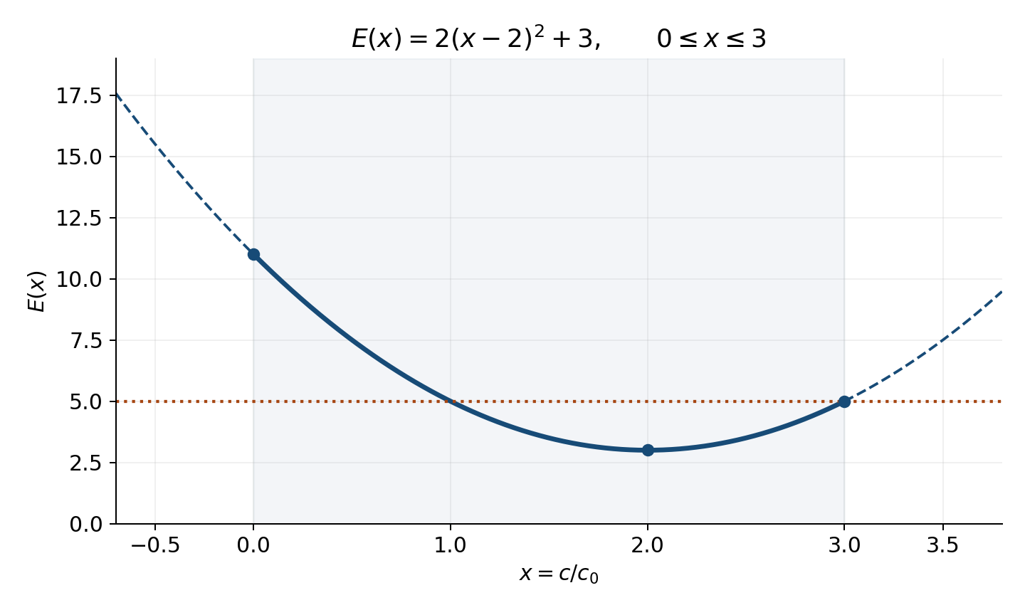
1. The coefficient of the square is positive, so the parabola opens upward. Its vertex is $(2,3)$. The admissible input domain is $[0,3]$, and the minimum penalty three is attained at $x=2$. On that domain, $|x-2|\le2$, so $E(x)\le11$, with equality at $x=0$. Every value between three and eleven occurs: for $e\in[3,11]$, the input $x=2-\sqrt{(e-3)/2}$ lies in $[0,2]$ and has penalty $e$. Therefore the admissible range is exactly $[3,11]$. The unrestricted polynomial instead has domain $\mathbb R$ and range $[3,\infty)$; the scientific restriction must not be inferred from the polynomial alone.

2. The solid curve lies on or below the horizontal boundary between the two crossings. Algebraically,

   $$E(x)\le5\iff 2(x-2)^2\le2\iff |x-2|\le1\iff1\le x\le3.$$

   Intersecting with the admissible domain leaves $[1,3]$. Both endpoints are included because each has penalty exactly five and the requested comparison is non-strict. At $x=0$ the penalty is eleven, so that endpoint is not accepted by this tolerance.

3. Solving $E(x)=5$ gives $x=1$ or $x=3$, both admissible. The original model is not injective: distinct concentrations on opposite sides of the vertex can have the same penalty. Restricting inputs to $[2,3]$ makes the penalty strictly increasing, with range $[3,5]$. Its inverse is

   $$x=2+\sqrt{\frac{e-3}{2}},\qquad 3\le e\le5.$$

   The positive branch is selected by $x\ge2$; it is not a rule that square-root equations have only one candidate. Alternatively, restricting to $[0,2]$ gives the negative branch and inverse domain $[3,11]$. Returning to physical concentration requires $c=c_0x$.

4. The dashed continuation shows values of the polynomial, not an enlarged scientific operating domain. Negative $x$ would violate nonnegative concentration, and $x>3$ would exceed the stated instrument range. A real value of $E(x)$ at such an input establishes algebraic definability, not physical admissibility or calibration validity.

Summary

Factors reveal roots and sign changes, while repeated roots require separate zero cases. Completing squares derives quadratic roots, extrema and geometric forms. Rational exclusions survive cancellation. Coordinate equations describe loci that need not be single-valued functions. Finite geometric sums provide exact discrete accumulation without introducing differential or integral calculus.