Polar Coordinates and Complex Numbers

Motivation

You need rectangular coordinates, radians, elementary trigonometric identities and algebra. This chapter adds two genuinely new structures to the earlier coordinate chapters: polar descriptions of points and arithmetic with complex numbers. You should be able to convert coordinates with the correct quadrant, interpret simple polar loci, compute with complex numbers in rectangular and polar form, and find all roots of a simple complex power equation.

A point, a vector and a complex number can all be represented by a pair of real numbers. Their interpretations are not identical. Polar coordinates describe the same plane with distance and direction; complex arithmetic adds a multiplication that encodes scaling and rotation.

8.1 Polar coordinates and their nonuniqueness

Definition

Fix an origin and a positive horizontal axis. A pair $(r,\theta)$ of polar coordinates describes the rectangular point

$$x=r\cos\theta,\qquad y=r\sin\theta.$$

Our default convention is $r\ge0$ and angles in radians. For $r>0$, $r$ is distance from the origin and $\theta$ is direction measured counterclockwise from the positive horizontal axis. The same point has coordinates $(r,\theta+2k\pi)$ for every integer $k$. At $r=0$, every angle gives the origin, so the point has no unique direction.

Some texts permit signed radii. Under that convention,

$$(r,\theta)\quad\text{and}\quad(-r,\theta+\pi)$$

describe the same point. A negative radius means travel in the direction opposite to the stated angle. It is not a negative distance. We will say explicitly when signed-radius descriptions are allowed; otherwise $r\ge0$.

Worked example

Worked example 1: from polar to rectangular. At $(r,\theta)=(4,5\pi/6)$,

$$x=4(-\sqrt3/2)=-2\sqrt3,\qquad y=4(1/2)=2.$$

The point is in quadrant II and has squared distance $12+4=16$, as required. With signed radii it could also be represented as $(-4,-\pi/6)$.

8.2 Recovering the angle without losing the quadrant

Given a nonzero point $(x,y)$, its nonnegative radius is

$$r=\sqrt{x^2+y^2}>0.$$

The angle must satisfy both $\cos\theta=x/r$ and $\sin\theta=y/r$. If $x\ne0$, $\tan\theta=y/x$ is a useful intermediate equation, but tangent has period $\pi$, so it cannot distinguish opposite directions. A principal angle can be chosen in $(-\pi,\pi]$; this convention includes $\pi$ and excludes $-\pi$.

Use the signs of $x,y$ to select the quadrant, then add multiples of $2\pi$ for other representations. If $x=0$ and $y>0$, choose $\theta=\pi/2$; if $x=0$ and $y<0$, choose $\theta=-\pi/2$. At the origin the radius is zero and no unique angle exists.

Worked example

Worked example 2: a quadrant trap. For $(x,y)=(-\sqrt3,-1)$, $r=2$. The ratio $y/x=1/\sqrt3$ gives reference angle $\pi/6$. Both components are negative, so the point lies in quadrant III. A principal angle is $-5\pi/6$, not $\pi/6$. Thus $(2,-5\pi/6)$ is a valid principal polar representation. The expression $\arctan(y/x)$ alone would have returned a direction in quadrant I.

For a general nonzero point, an angle can be given exactly by its sine and cosine when no familiar special angle applies. A two-argument angle routine can encode the quadrant, but its output interval and its treatment of $(0,0)$ still need checking.

8.3 Loci and transformations between coordinate systems

The identities

$$r^2=x^2+y^2,\qquad r\cos\theta=x,\qquad r\sin\theta=y$$

connect the two systems. They are especially useful for equations of curves. Converting an equation means preserving the set of points, including possible points at the origin. Dividing by $r$ can remove the origin; multiplying by $r$ can introduce it unless checked.

For $R>0$, the equation $r=R$ is the circle $x^2+y^2=R^2$. A fixed direction $\theta=\alpha$, with $r\ge0$, is a ray from the origin, not a complete line. The union of the opposite rays $\theta=\alpha$ and $\theta=\alpha+\pi$ is a line through the origin. If signed radii are allowed, one fixed angle with all real radii describes that full line.

Worked example

Worked example 3: a circle described by a variable radius. Consider $r=4\cos\theta$ with $r\ge0$. Multiply by $r$ to obtain

$$r^2=4r\cos\theta\quad\implies\quad x^2+y^2=4x,$$

or $(x-2)^2+y^2=4$. This is a circle of centre $(2,0)$ and radius two. Check the converse: for a nonzero point on this circle, $r>0$ and division by $r$ gives $r=4\cos\theta$. The origin is also on the polar locus, since $r=0$ works at $\theta=\pi/2$. Hence the conversion has neither lost nor added a point. Under the nonnegative-radius convention, angles with $\cos\theta<0$ have no allowed radius for this equation; they are not extra points on the opposite side.

Worked example

Worked example 4: a line and a forbidden division. The line $x=-2$ becomes $r\cos\theta=-2$. Solving for $r$ gives $r=-2/\cos\theta$, but only when $\cos\theta\ne0$ and, for our convention, $\cos\theta<0$. No point on the line has $r=0$. The equation is not a ray merely because polar variables appear in it; $\theta$ varies through the appropriate left-facing directions.

Common mistake

A graph is a visual aid, not a substitute for these domain checks. When converting an inequality, the sign of a factor used for multiplication matters just as it does in one-variable algebra.

8.4 Complex arithmetic in rectangular form

Definition

A complex number has form $z=a+bi$, where $a,b\in\mathbb R$ and $i^2=-1$. Its real and imaginary parts are $\operatorname{Re}z=a$ and $\operatorname{Im}z=b$. The imaginary part is the real coefficient $b$, not $bi$. Equality means equality of both components.

One can define complex numbers rigorously as pairs: $(a,b)+(c,d)=(a+c,b+d)$ and $(a,b)(c,d)=(ac-bd,ad+bc)$. Identifying $(a,0)$ with the real number $a$ and $(0,1)$ with $i$ gives the rules above. Thus ordinary distributive expansion remains valid, with each $i^2$ replaced by $-1$:

$$(a+bi)(c+di)=(ac-bd)+(ad+bc)i.$$

Proof details: the algebra behind complex multiplication

The pair definition in Section 8.4 uses only real arithmetic. Here are the laws needed by the subsequent proofs, checked without presupposing complex distributivity. Write $z=(a,b)$, $w=(c,d)$ and $u=(e,f)$, with all six coordinates real. Addition is associative and commutative component by component, its identity is $(0,0)$, and the additive inverse of $(a,b)$ is $(-a,-b)$. The real equalities $ac=ca$ and $ad+bc=cb+da$ show that multiplication is commutative, and its identity is $(1,0)$.

For distributivity, expand the pair definition:

$$z(w+u)=(a(c+e)-b(d+f),\ a(d+f)+b(c+e))=zw+zu.$$

For associativity, both $(zw)u$ and $z(wu)$ expand, using real distributivity, to the same pair

$$(ace-bde-adf-bcf,\ acf-bdf+ade+bce).$$

Thus regrouping and distributive factorization in later complex calculations are justified. In particular $i=(0,1)$ has square $(-1,0)$, and the embedding $a\mapsto(a,0)$ preserves real sums, products and one.

For $w=(c,d)\ne(0,0)$, the positive real number $q=c^2+d^2$ gives

$$(c,d)\left(\frac c q,-\frac d q\right) =\left(\frac{c^2+d^2}{q},\frac{-cd+dc}{q}\right)=(1,0).$$

Commutativity proves the product in the other order too. This proves the inverse first; division $z/w$ is then defined as $zw^{-1}$, yielding Section 8.5's quotient formula. If $zw=0$ and $z\ne0$, associativity gives $w=(z^{-1}z)w=z^{-1}(zw)=0$, proving the zero-product property used in the quadratic factorization. This is not an assumption imported from the real numbers.

For $z=a+bi$ and $w=c+di$, the same multiplication formula gives

$$\overline{zw}=(ac-bd)-(ad+bc)i=(a-bi)(c-di)=\bar z\bar w, \qquad \overline{z+w}=(a+c)-(b+d)i=\bar z+\bar w.$$

Finally, applying that formula to the two trigonometric pairs yields

$$\begin{aligned} (\cos\alpha+i\sin\alpha)(\cos\beta+i\sin\beta) &=(\cos\alpha\cos\beta-\sin\alpha\sin\beta)\\ &\quad+i(\cos\alpha\sin\beta+\sin\alpha\cos\beta)\\ &=\cos(\alpha+\beta)+i\sin(\alpha+\beta). \end{aligned}$$

The last equality uses the real angle-addition identities. It supplies the multiplication rule used in Section 8.6, without requiring a definition of the complex exponential or an order on complex numbers.

Complex numbers contain the reals, but there is no ordering of all complex numbers compatible with the usual ordered-field rules. Such an order would make every nonzero square positive, including $i^2=-1$, contradicting the positivity of one. Statements such as $z>0$ therefore have no default meaning for arbitrary complex $z$.

Worked example

Worked example 5: multiply and solve. First,

$$(2-3i)(1+4i)=2+8i-3i-12i^2=14+5i.$$

Next, $z^2+2z+5=0$ is equivalent to $(z+1)^2=-4$, giving $z=-1+2i$ or $z=-1-2i$. These are all solutions, because

$$(z+1)^2+4=(z+1-2i)(z+1+2i)$$

and a product in $\mathbb C$ is zero only when one factor is zero. That zero-product property follows from the existence of inverses for nonzero complex numbers, derived next. There are no real roots, but “no real roots” does not mean “no complex roots.”

8.5 Conjugate, modulus and division

The conjugate of $z=a+bi$ is $\bar z=a-bi$. Its modulus is the nonnegative real number

$$|z|=\sqrt{a^2+b^2}.$$

Direct calculation gives $z\bar z=a^2+b^2=|z|^2$, so $|z|=0$ exactly when $z=0$. Also $z+\bar z=2\operatorname{Re}z$ and $z-\bar z=2i\operatorname{Im}z$.

If $w=c+di\ne0$, then $c^2+d^2>0$ and

$$\frac zw=\frac{z\bar w}{w\bar w} =\frac{(ac+bd)+(bc-ad)i}{c^2+d^2}.$$

In particular, $w^{-1}=\bar w/|w|^2$. Multiplying by $w$ verifies the inverse, so division by a nonzero complex number is legitimate. There is still no division by zero.

Worked example

Worked example 6: a complex quotient. Calculate

$$\frac{3+2i}{1-i} =\frac{(3+2i)(1+i)}2 =\frac{1+5i}{2}.$$

Multiplication by $1-i$ checks that this recovers $3+2i$. Multiplying only the denominator by a conjugate would change the number; numerator and denominator must receive the same nonzero factor.

Proposition

Expansion also proves $\overline{zw}=\bar z\bar w$ and $\overline{z+w}=\bar z+\bar w$. Hence

$$|zw|^2=zw\overline{zw}=(z\bar z)(w\bar w)=|z|^2|w|^2.$$

Taking nonnegative square roots gives $|zw|=|z||w|$, and for $w\ne0$, $|z/w|=|z|/|w|$. The modulus is a real distance, not a new order relation on complex numbers.

Proof

For $z=a+bi$ and $w=c+di$, Chapter 7's two-dimensional inequality gives $ac+bd\le|z||w|$. Therefore

$$|z+w|^2=|z|^2+|w|^2+2(ac+bd)\le(|z|+|w|)^2,$$

and taking square roots proves the complex triangle inequality $|z+w|\le|z|+|w|$.

8.6 Complex polar form and multiplication

Identify $z=a+bi$ with the plane point $(a,b)$. For $z\ne0$, let $r=|z|>0$ and choose an argument $\theta$ satisfying $\cos\theta=a/r$, $\sin\theta=b/r$. Write

$$z=r(\cos\theta+i\sin\theta)=r\,\operatorname{cis}\theta,$$

where $\operatorname{cis}\theta$ is only an abbreviation for $\cos\theta+i\sin\theta$. Every argument differs by an integer multiple of $2\pi$. The principal argument, denoted here $\operatorname{Arg}z$, is chosen in $(-\pi,\pi]$. Zero has modulus zero but no defined argument. We do not need a complex exponential definition in this chapter.

Using distributivity and the angle-addition identities,

$$\operatorname{cis}\alpha\,\operatorname{cis}\beta =\operatorname{cis}(\alpha+\beta).$$

Thus, for positive radii $r,s$,

$$(r\operatorname{cis}\alpha)(s\operatorname{cis}\beta) =rs\operatorname{cis}(\alpha+\beta),$$

and division by the second nonzero number gives radius $r/s$ and angle $\alpha-\beta$. Multiplication scales distances and adds directions. A principal argument of a product may require adding or subtracting $2\pi$; principal arguments do not always add as ordinary real numbers without adjustment.

Worked example

Worked example 7: multiplication as a transformation. Multiplication by $1+i=\sqrt2\operatorname{cis}(\pi/4)$ scales every distance from the origin by $\sqrt2$ and rotates every nonzero point counterclockwise by $\pi/4$. For $z=2-i$,

$$(1+i)(2-i)=3+i.$$

The original modulus is $\sqrt5$ and the new one $\sqrt{10}$, confirming the scale factor. The transformation sends zero to zero, although no angle is assigned to zero.

For a nonnegative integer $n$, repeated multiplication gives de Moivre's formula

$$(\operatorname{cis}\theta)^n=\operatorname{cis}(n\theta).$$

Its base $n=0$ is one, and its induction step is the two-angle multiplication rule. For negative integers it remains true because $\operatorname{cis}\theta$ has inverse $\operatorname{cis}(-\theta)$. Consequently, for nonzero $z=r\operatorname{cis}\theta$ and any integer $n$,

$$z^n=r^n\operatorname{cis}(n\theta).$$

For $z=0$, positive integer powers are zero; zero and negative exponents are not assigned by this statement.

Worked example

Worked example 8: a power without a long expansion. Since $1+i=\sqrt2\operatorname{cis}(\pi/4)$,

$$(1+i)^6=(\sqrt2)^6\operatorname{cis}(3\pi/2)=-8i.$$

The angle is $6\pi/4=3\pi/2$, not $3\pi$. As an independent check, $(1+i)^2=2i$, so the sixth power is $(2i)^3=-8i$. Multiplying angles correctly matters as much as finding a radius.

In the complete ordered real field, for $b>0$ and integer $m\ge1$, let $S=\{t\ge0:t^m\le b\}$. It contains $\min\{1,b\}>0$ and is bounded above by $\max\{1,b\}$, so $r=\sup S>0$ exists. Finite factorization gives, for nonnegative $t,r\le M$,

$$t^m-r^m=(t-r)\sum_{j=0}^{m-1}t^{m-1-j}r^j,\qquad |t^m-r^m|\le mM^{m-1}|t-r|.$$

Take $M=r+1$. If $r^m<b$, choose $0<h<1$ so $mM^{m-1}h<b-r^m$; then $(r+h)^m<b$, contradicting the upper bound $r$. If $r^m>b$, choose $0<h<\min\{1,r\}$ with $mM^{m-1}h<r^m-b$. Then $(r-h)^m>b$, and monotonicity of integer powers on nonnegative numbers makes $r-h$ an upper bound of $S$, contradicting its supremum. Hence $r^m=b$. At $b=0$ the unique nonnegative root is zero. The same factorization shows $t^m>s^m$ whenever $t>s\ge0$, so this positive root is unique.

8.7 Finding every root of a complex power

Proposition

Let $n\ge1$ be an integer and $w=R\operatorname{cis}\phi\ne0$, where $R>0$. To solve $z^n=w$, a root must be nonzero. Write it as $z=r\operatorname{cis}\theta$. Modulus and argument comparisons give

$$r^n=R,\qquad n\theta=\phi+2k\pi\quad(k\in\mathbb Z).$$

Because $r>0$, the radius is uniquely $R^{1/n}$. The roots are

$$z_k=R^{1/n}\operatorname{cis}\left(\frac{\phi+2k\pi}{n}\right), \qquad k=0,1,\ldots,n-1.$$

They are distinct: two listed angles differ by $2\pi(k-j)/n$, which is a multiple of $2\pi$ only when $k=j$ within this range. Every integer $k$ reduces to one of these cases modulo $n$, so the list is complete. The roots are equally spaced on a circle. Changing the chosen argument $\phi$ merely permutes the same roots. If $w=0$, the equation has only the single root zero, not $n$ distinct roots.

Worked example

Worked example 9: cube roots of a negative real number. Write $-8=8\operatorname{cis}\pi$. The three cube roots have radius two and arguments $\pi/3$, $\pi$, $5\pi/3$. In rectangular form they are

$$1+i\sqrt3,\qquad -2,\qquad 1-i\sqrt3.$$

Cubing any of them multiplies its argument by three and cubes the radius, giving $-8$. For instance, $(1+i\sqrt3)^2=-2+2i\sqrt3$, and multiplying once more gives $-8$. The real cube root $-2$ is one member, not the entire complex solution set.

8.8 Geometric equations in complex notation

Because $|z-z_0|$ is the rectangular distance between the points represented by $z$ and $z_0$, the equation $|z-z_0|=R$ with $R>0$ is a circle. If $R=0$ it is the single point $z_0$; if $R<0$ it has no solutions.

Worked example

Worked example 10: equal-distance locus. For $z=x+iy$,

$$|z-1|=|z+1|$$

compares distances from $(1,0)$ and $(-1,0)$. Both sides are nonnegative, so squaring preserves equivalence:

$$(x-1)^2+y^2=(x+1)^2+y^2\iff -4x=0.$$

Thus the locus is the imaginary axis $x=0$. This is its own algebraic proof of the perpendicular-bisector picture; a diagram alone would not show that all points have been found.

8.9 Graded exercises

Foundation

Checkpoint

Exercise 1

1. Convert $(r,\theta)=(6,2\pi/3)$ to rectangular coordinates.

Checkpoint

Exercise 2

2. Find a principal polar representation of $(x,y)=(1,-\sqrt3)$, using $r\ge0$ and $-\pi<\theta\le\pi$.

Checkpoint

Exercise 3

3. Give two polar descriptions of the origin and explain why neither is its unique direction.

Checkpoint

Exercise 4

4. Compute $(3-2i)+(1+5i)$, $(3-2i)(1+5i)$ and $i^{2026}$.

Checkpoint

Exercise 5

5. For $z=-3+4i$, find $\bar z$, $|z|$, $z\bar z$, $\operatorname{Re}z$ and $\operatorname{Im}z$.

Core

Checkpoint

Exercise 6

6. Convert $r=2\sin\theta$, $r\ge0$, to a rectangular locus. Check the origin separately.

Checkpoint

Exercise 7

7. Does $\theta=\pi/3$ with $r\ge0$ describe a line or a ray? State a rectangular equation and an extra inequality describing exactly the same set.

Checkpoint

Exercise 8

8. Calculate $(2-i)/(1+2i)$ and check by multiplication.

Checkpoint

Exercise 9

9. Solve $z^2-4z+13=0$ over $\mathbb C$.

Checkpoint

Exercise 10

10. Solve $z+2\bar z=3+4i$ by writing $z=x+iy$.

Checkpoint

Exercise 11

11. Find the principal argument of $(\operatorname{cis}(3\pi/4))^2$. Explain why the sum of two principal arguments needs adjustment.

Checkpoint

Exercise 12

12. Compute $(\sqrt3+i)^4$ exactly in rectangular form.

Checkpoint

Exercise 13

13. Find all fourth roots of $-16$, in both polar and rectangular form.

Checkpoint

Exercise 14

14. Find the complete locus $|z-(1+i)|=2$ and give its rectangular equation.

Checkpoint

Exercise 15

15. Write $(1+i)/(\sqrt3-i)$ in polar form and rectangular form.

Synthesis

Checkpoint

Exercise 16

16. Prove $\operatorname{Re}z=(z+\bar z)/2$ and $\operatorname{Im}z=(z-\bar z)/(2i)$. Explain why these formulas do not make an arbitrary complex number ordered.

Checkpoint

Exercise 17

17. Let $\omega=\operatorname{cis}(2\pi/3)$. Prove $1+\omega+\omega^2=0$ and list all solutions of $z^3=1$.

Checkpoint

Exercise 18

18. A transformation sends $z$ to $(1-i)z+2$. Describe its scale, rotation and translation in that order. Find the image of $i$.

Checkpoint

Exercise 19

19. Prove $|z+w|\ge\big||z|-|w|\big|$ for complex $z,w$ using the triangle inequality. Use it to bound the modulus of a sum with $|z|=5$, $|w|=2$.

Checkpoint

Exercise 20

20. A student cancels $r$ in $r^2=3r\cos\theta$ and concludes that the two equations have the same polar-coordinate pairs. What has been lost at $r=0$? Do the two equations nevertheless describe the same rectangular point set? Justify both answers.

8.10 Full solutions

Solution · Exercise 1

1. The point is $(6(-1/2),6(\sqrt3/2))=(-3,3\sqrt3)$. Its squared distance is $9+27=36$.

Solution · Exercise 2

2. The radius is two. The point is in quadrant IV with cosine $1/2$ and sine $-\sqrt3/2$, so its principal angle is $-\pi/3$. A representation is $(2,-\pi/3)$.

Solution · Exercise 3

3. Both $(0,0)$ and $(0,\pi/2)$ give $(x,y)=(0,0)$. Indeed every angle does. The angle coordinate is arbitrary at zero, not an assigned geometric direction.

Solution · Exercise 4

4. The sum is $4+3i$. The product is $3+15i-2i-10i^2=13+13i$. Since powers of $i$ repeat every four and $2026=4(506)+2$, $i^{2026}=i^2=-1$.

Solution · Exercise 5

5. The conjugate is $-3-4i$, modulus five, product with its conjugate $25$, real part $-3$ and imaginary part $4$.

Solution · Exercise 6

6. Multiplication by $r$ gives $r^2=2r\sin\theta$, hence $x^2+y^2=2y$ or $x^2+(y-1)^2=1$. For any nonzero point on this circle, divide by its positive radius to recover the polar equation. The origin is allowed because $r=0$, $\theta=0$ satisfies $r=2\sin\theta$. Thus the point set is exactly that circle.

Solution · Exercise 7

7. It is a ray. Its rectangular description is $y=\sqrt3x$ with $x\ge0$. The origin is included. The equation without the inequality would also include the opposite ray.

Solution · Exercise 8

8. Multiplication by the conjugate gives $(2-i)(1-2i)/5=(-5i)/5=-i$. Checking, $(1+2i)(-i)=2-i$.

Solution · Exercise 9

9. Complete the square: $(z-2)^2=-9$. Thus $z=2\pm3i$. Factoring $(z-2-3i)(z-2+3i)$ verifies both roots and completeness.

Solution · Exercise 10

10. With $z=x+iy$, $z+2\bar z=3x-iy$. Equating components yields $x=1$ and $y=-4$, so $z=1-4i$. Direct substitution gives $(1-4i)+2(1+4i)=3+4i$.

Solution · Exercise 11

11. The product is $\operatorname{cis}(3\pi/2)$, whose principal argument is $-\pi/2$ in the chosen interval. The ordinary sum $3\pi/2$ is a valid argument but not the principal one.

Solution · Exercise 12

12. Here $\sqrt3+i=2\operatorname{cis}(\pi/6)$. Its fourth power is $16\operatorname{cis}(2\pi/3)=-8+8\sqrt3i$. As a check, its square is $2+2\sqrt3i$ and squaring again gives the same result.

Solution · Exercise 13

13. The radius is two and angles are $\pi/4$, $3\pi/4$, $5\pi/4$, $7\pi/4$. The rectangular roots are $\sqrt2+i\sqrt2$, $-\sqrt2+i\sqrt2$, $-\sqrt2-i\sqrt2$, $\sqrt2-i\sqrt2$. There are four distinct roots, and each fourth power has modulus $16$ and argument equal to an odd multiple of $\pi$.

Solution · Exercise 14

14. It is the circle of centre $(1,1)$ and radius two, with equation $(x-1)^2+(y-1)^2=4$ for $z=x+iy$. No points have been added by squaring because a modulus and the stated radius are nonnegative.

Solution · Exercise 15

15. The numerator has modulus $\sqrt2$ and argument $\pi/4$; the denominator has modulus two and argument $-\pi/6$. Thus the quotient is $(1/\sqrt2)\operatorname{cis}(5\pi/12)$. Rectangular multiplication by $\sqrt3+i$ gives $[(\sqrt3-1)+i(\sqrt3+1)]/4$. Its squared modulus is $[(\sqrt3-1)^2+(\sqrt3+1)^2]/16=1/2$, agreeing with the polar radius.

Solution · Exercise 16

16. Write $z=a+bi$. Its sum with its conjugate is $2a$, and their difference is $2bi$, giving both formulas. They extract real component values, but they do not define a compatible order for all complex numbers. The contradiction from $i^2=-1$ remains.

Solution · Exercise 17

17. We have $\omega^3=\operatorname{cis}(2\pi)=1$ and $\omega\ne1$. The finite factorization $(\omega-1)(1+\omega+\omega^2)=\omega^3-1=0$ permits division by the nonzero factor $\omega-1$, proving the sum is zero. The complete cubic-root formula gives $1,\omega,\omega^2$ as all solutions of $z^3=1$.

Solution · Exercise 18

18. Multiplication by $1-i=\sqrt2\operatorname{cis}(-\pi/4)$ scales by $\sqrt2$ and rotates clockwise through $\pi/4$. Adding two then translates two units in the positive real direction. The image of $i$ is $(1-i)i+2=3+i$. Translation occurs after the multiplication; reversing the order would generally change the map.

Solution · Exercise 19

19. The triangle inequality gives $|z|=|(z+w)-w|\le|z+w|+|w|$, hence $|z|-|w|\le|z+w|$. Interchanging $z,w$ gives the other bound, so the absolute difference of moduli is a lower bound. Together with the ordinary upper bound, $3\le|z+w|\le7$ when the moduli are five and two. Both endpoints can occur, with opposite or matching directions respectively.

Solution · Exercise 20

20. At $r=0$, the original equation $r^2=3r\cos\theta$ holds for every angle. The cancelled equation $r=3\cos\theta$ holds at $r=0$ only for angles with $\cos\theta=0$. Thus many polar-coordinate pairs are lost. Nevertheless they all describe the same origin, which remains represented, for example at $(0,\pi/2)$. At every nonzero radius division is reversible. Both therefore describe the same rectangular point set, the circle $(x-3/2)^2+y^2=9/4$, despite having different sets of coordinate pairs.

Graphical workshop G3

Checkpoint

Graphical problem G3: circle and origin

Polar pairs, a circle and the origin

Let $r,x,y$ be numerical lengths measured in centimetres, and let $\theta$ be in radians. Use nonnegative polar radii and

$$x=r\cos\theta,\qquad y=r\sin\theta.$$

Consider the polar equation

$$r=4\cos\theta,\qquad r\ge0.$$

The figure uses equal scales on the two rectangular axes. The ray through $P$ has direction $\theta=\pi/3$.

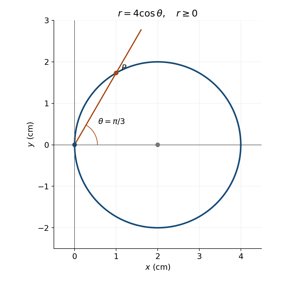
1. Convert the polar equation to a rectangular equation. Verify the centre and radius read from the graph. Prove the converse and check the origin separately, so that the full point set is established.

Solution · Graphical problem G3: circle and origin

1. Multiplying by $r$ gives $r^2=4r\cos\theta$, hence

   $$x^2+y^2=4x\iff(x-2)^2+y^2=4.$$

   The centre is $(2,0)$ centimetres and the radius is two centimetres, matching the undistorted circle in the figure. Multiplication alone proves only one implication. Conversely, take a nonzero point satisfying the rectangular equation, choose its nonnegative radius $r=\sqrt{x^2+y^2}>0$ and a corresponding angle. Then $r^2=4r\cos\theta$, and division by this positive radius recovers $r=4\cos\theta$. The origin also belongs to the polar locus: $r=0$, $\theta=\pi/2$ satisfies the equation. Thus no rectangular point was lost or added.

Continue with the complete G3 graphical practice, including all four questions and full solutions.

Summary

Polar conversion requires a radius convention and a quadrant-aware angle. Multiple coordinate pairs can represent one point, especially at the origin. Complex addition and multiplication are defined componentwise through distributivity and $i^2=-1$; division uses a nonzero conjugate product. Moduli give real distances. In complex polar form multiplication adds arguments, powers multiply them, and a nonzero number has exactly $n$ distinct $n$th roots. Principal arguments need branch adjustment, and zero has no argument. Complex distances turn many locus problems back into rectangular geometry.

Connections. Rectangular coordinates and trigonometry come from Chapters 2–3; the present chapter develops polar coordinates and complex arithmetic. Chapter 7's inequalities and induction justify modulus estimates and integer powers. Finite geometric factorization from Chapter 5 explains simple roots-of-unity identities.