5.3 Delta-epsilon limits, limit laws, and continuity

From sequence limits to function limits

For sequences, the definition of

$$\lim_{n\to\infty}x_n=L$$

said that every small tolerance around $L$ can be achieved by going far enough out in the sequence.

For functions, we want an analogous sentence:

as $x$ approaches $a$, the function value $f(x)$ approaches $L$.

But now “going far enough out” no longer makes sense. We need a new way to say that $x$ is close enough to $a$. That role is played by $\delta$.

Open intervals and punctured domains

Definition 5.3.1

(Open interval)

An open interval is a subset of $R$ of one of the forms

$$(b,c)=\{x\in R\mid b\lt x\lt c\},$$$$(-\infty,c)=\{x\in R\mid x\lt c\},$$$$(b,\infty)=\{x\in R\mid b\lt x\},$$

where $b,c\in R$ and $b\lt c$.

To define a limit at a point $a$, consider functions defined on an open interval with the point $a$ removed. That removal is important: a limit is about what happens near $a$, not necessarily what happens at $a$.

The formal delta-epsilon definition

Definition 5.3.2

(Limit of a function at a point)

Suppose $I$ is an open interval containing $a\in R$, and let $f:I\setminus\{a\}\to R$. We say

$$\lim_{x\to a}f(x)=L$$

if and only if for every $\varepsilon\gt0$, there exists $\delta\gt0$ such that

$$0\lt|x-a|\lt\delta \implies |f(x)-L|\lt\varepsilon.$$

The implication is required for every $x\in I\setminus\{a\}$. The number $\delta$ may depend on $\varepsilon$, but not on the input $x$.

Read the implication carefully:

• $0\lt|x-a|\lt\delta$ means $x$ is close to $a$, but not equal to $a$;
• $|f(x)-L|\lt\varepsilon$ means the function value lands inside the $\varepsilon$-band around $L$.

So the definition says:

Every requested output accuracy $\varepsilon$ can be guaranteed by forcing the input $x$ into a sufficiently small punctured neighborhood of $a$.

Common mistake

(The limit definition ignores the value at a)

The condition $0\lt|x-a|$ removes the point $a$ itself. So $f(a)$ may be undefined, or may differ from $L$, while the limit still exists.

First example: $\lim\limits_{x\to 3}(2x+1)=7$

The basic linear test case is the function $f(x)=2x+1$ at $a=3$.

Worked example 5.3.3

(Choosing $\delta=\varepsilon/2$)

Let $f(x)=2x+1$, $a=3$, and $L=7$. Then

$$|f(x)-7| = |(2x+1)-7| = |2x-6| = 2|x-3|.$$

So in order to force $|f(x)-7|\lt\varepsilon$, it is enough to make

$$|x-3|\lt\frac{\varepsilon}{2}.$$

Therefore choose

$$\delta=\frac{\varepsilon}{2}.$$

Then whenever $0\lt|x-3|\lt\delta$,

$$|f(x)-7|=2|x-3|\lt2\delta=2\cdot \frac{\varepsilon}{2}=\varepsilon.$$

Hence

$$\lim_{x\to 3}(2x+1)=7.$$

This example shows the standard proof pattern:

1. start with $|f(x)-L|$,
2. simplify it into an expression involving $|x-a|$,
3. choose $\delta$ to make that expression smaller than $\varepsilon$.

Two more basic examples

Worked example 5.3.4

(Constant functions)

If $f(x)=c$ for all $x$, then

$$|f(x)-c|=|c-c|=0\lt\varepsilon$$

for every $\varepsilon\gt0$ and every $x$.

So any positive number can be chosen as $\delta$, and

$$\lim_{x\to a}c=c.$$

Worked example 5.3.5

(A function with a hole)

Consider

$$f:(0,\infty)\setminus\{2\}\to R,\qquad f(x)=\frac{x^2-4}{x-2}.$$

The formula is undefined at $x=2$, but for $x\ne 2$ it simplifies to

$$f(x)=x+2.$$

So near $x=2$,

$$|f(x)-4|=|(x+2)-4|=|x-2|.$$

Therefore choosing $\delta=\varepsilon$ works. If $0\lt|x-2|\lt\delta$, then

$$|f(x)-4|\lt\varepsilon.$$

Hence

$$\lim_{x\to 2}\frac{x^2-4}{x-2}=4,$$

even though $f(2)$ is not defined.

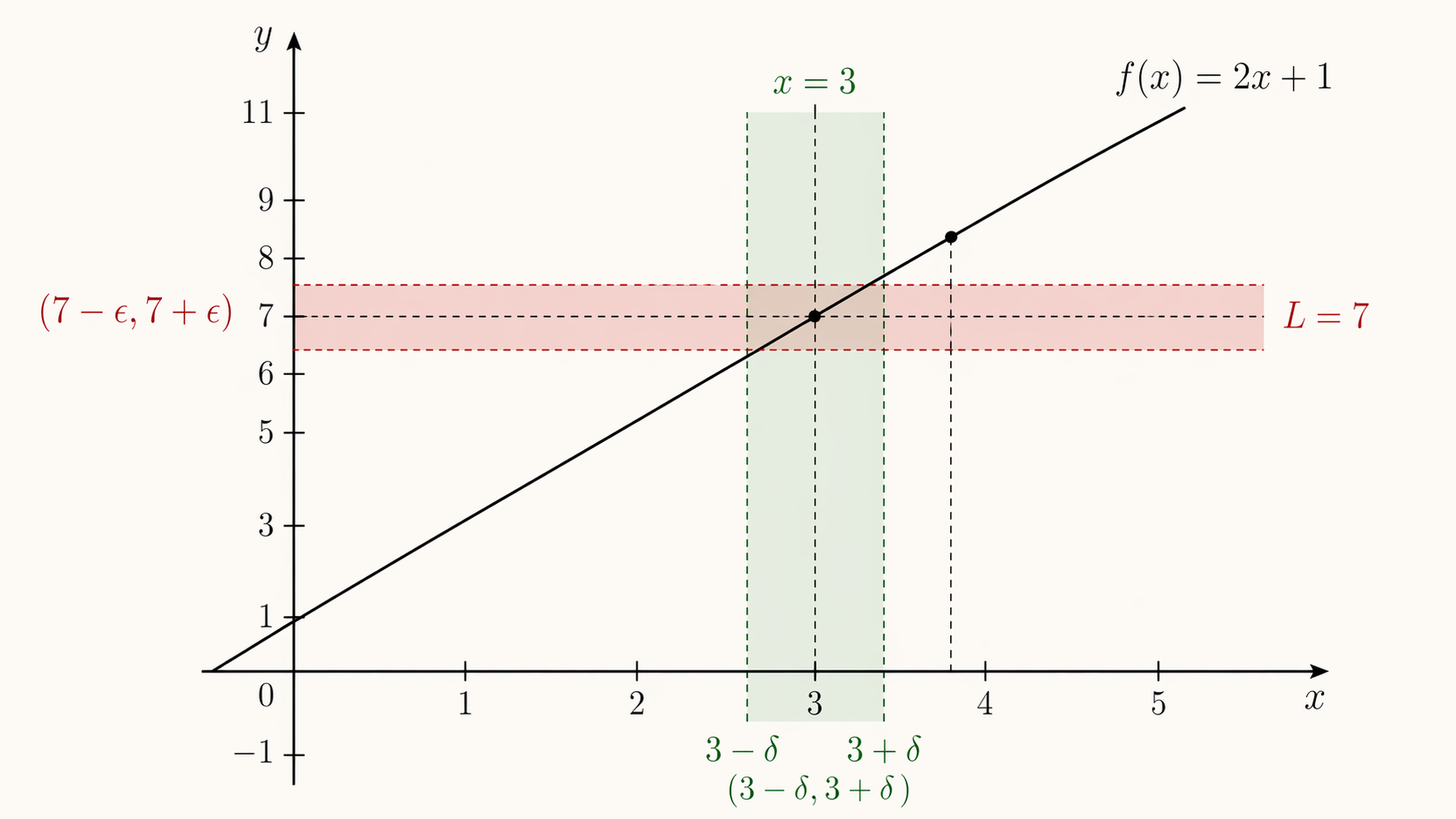
Figure. The $\delta$-$\varepsilon$ definition links an input neighborhood of $a$ to an output band around $L$. The proof task is to choose $\delta$ so that this implication always succeeds.

Explore the definition interactively

The explorer below lets you choose one of the examples, select $\varepsilon$, and test sample inputs $x$. The point is to see the implication

$$0\lt|x-a|\lt\delta \implies |f(x)-L|\lt\varepsilon$$

as a relationship between an input strip and an output band.

How limits can fail to exist

To rule out a proposed limit $L$, one must find a fixed $\varepsilon\gt0$ such that every $\delta>0$ admits some $x\in I\setminus\{a\}$ with $0\lt|x-a|\lt\delta$ and

$$|f(x)-L|\ge \varepsilon.$$

To prove that no limit exists, this rejection must work for every real candidate $L$.

Consider

$$f(x)=\frac{|x|}{x},$$

which equals $1$ for $x\gt0$ and $-1$ for $x\lt0$.

Worked example 5.3.6

(Why $|x|/x$ has no limit at $0$)

Let $L\in R$ be arbitrary and take $\varepsilon=1$. For any $\delta\gt0$, choose

$$x_1=\frac{\delta}{2}\gt0, \qquad x_2=-\frac{\delta}{2}\lt0.$$

Then both satisfy $|x_i|\lt\delta$, but

$$f(x_1)=1,\qquad f(x_2)=-1.$$

If $L\ge0$, then $|f(x_2)-L|=|{-1}-L|\ge1$. If $L<0$, then $|f(x_1)-L|=|1-L|>1$. Thus every candidate $L$ fails at a point in every punctured neighborhood, so the function has no limit at $0$.

This example captures a common failure mode: left-hand and right-hand behavior do not agree.

Algebra of limits

Once some basic limits are known, limit laws show how to build new ones from old ones.

Theorem 5.3.7

(Limit laws)

If $\lim\limits_{x\to a}f(x)=L$ and $\lim\limits_{x\to a}g(x)=M$, then:

• $\lim\limits_{x\to a}(f(x)+g(x))=L+M$,
• $\lim\limits_{x\to a}(f(x)g(x))=LM$,
• if $M\ne 0$, then

$$\lim_{x\to a}\frac{f(x)}{g(x)}=\frac{L}{M}.$$

One neighborhood for the sum law

The sum law illustrates the quantifier pattern in its shortest complete form. Suppose $f(x)→L$ and $g(x)→M$, and fix $\varepsilon\gt0$. The first limit supplies $\delta_f\gt0$ such that $|f(x)-L|\lt\varepsilon/2$ whenever $0\lt|x-a|\lt\delta_f$; the second supplies $\delta_g\gt0$ with the analogous bound for $g$. Set $\delta=\min(\delta_f,\delta_g)$. The same $x$ then satisfies both estimates, and therefore

$$\bigl|(f(x)+g(x))-(L+M)\bigr| \le |f(x)-L|+|g(x)-M| \lt\frac\varepsilon2+\frac\varepsilon2=\varepsilon.$$

The minimum is essential: it creates one neighborhood on which every required estimate holds simultaneously. A proof that chooses two unrelated input points, or that lets $\delta$ depend on $x$, has not established the quantified implication.

Proofs of the product and quotient laws

The product law is more than a symbolic rule: its proof must control two errors at once. Assume $f:I\setminus\{a\}\to R$ and $g:I\setminus\{a\}\to R$ have limits $L$ and $M$ at $a$, and let $\varepsilon\gt0$ be given. No value $f(a)$ is needed: every estimate below concerns the punctured domain. First use the limit of $f$ with tolerance $1$ to choose $\delta_0\gt0$ such that every $x\in I\setminus\{a\}$ with $0\lt|x-a|\lt\delta_0$ satisfies

$$|f(x)-L|\lt1,\qquad |f(x)|\lt|L|+1=:A.$$

Here $A\gt0$ is a local bound, obtained before the final epsilon budget. Choose $\delta_1$ so that every $x\in I\setminus\{a\}$ with $0\lt|x-a|\lt\delta_1$ gives $|g(x)-M|\lt\varepsilon/(2A)$. Choose $\delta_2$ so that every such $x$ with $0\lt|x-a|\lt\delta_2$ gives $|f(x)-L|\lt\varepsilon/(2B)$, where $B=\max(1,|M|)$. Set $\delta=\min(\delta_0,\delta_1,\delta_2)$. For any $x\in I\setminus\{a\}$ with $0\lt|x-a|\lt\delta$, all three estimates hold; the identity

$$f(x)g(x)-LM=f(x)(g(x)-M)+M(f(x)-L)$$

and the triangle inequality give

$$|f(x)g(x)-LM| \lt A\frac{\varepsilon}{2A}+|M|\frac{\varepsilon}{2B} \le\frac{\varepsilon}{2}+\frac{\varepsilon}{2}=\varepsilon.$$

This proves $f(x)g(x)→LM$, including the case $M=0$; the use of $B$ avoids dividing by zero in that case.

For the quotient, the assumption $M\ne0$ is essential. Since $g:I\setminus\{a\}\to R$ has limit $M$ at $a$, choose $\delta_0\gt0$ so that every $x\in I\setminus\{a\}$ with $0\lt|x-a|\lt\delta_0$ satisfies $|g(x)-M|\lt|M|/2$. Then

$$|g(x)|\ge |M|-|g(x)-M|\gt|M|/2.$$

On this same neighborhood, the reciprocal error satisfies

$$\left|\frac1{g(x)}-\frac1M\right| =\frac{|g(x)-M|}{|g(x)||M|} \le\frac{2|g(x)-M|}{|M|^2}.$$

Given $\varepsilon\gt0$, additionally choose $\delta_1$ so that every $x\in I\setminus\{a\}$ with $0\lt|x-a|\lt\delta_1$ satisfies $|g(x)-M|\lt\varepsilon|M|^2/2$; intersecting the two neighborhoods proves $1/g(x)→1/M$. Applying the product law to $f(x)$ and $1/g(x)$ now gives

$$\frac{f(x)}{g(x)}\longrightarrow \frac{L}{M}.$$

A local upper bound prevents multiplication from magnifying the error without control; a positive lower bound makes the reciprocal estimate possible.

The square-root limit used below is proved by rationalization in the exercises.

Worked example 5.3.8

(Using the sum law)

Consider $f(x)=2x+1$ and $g(x)=\sqrt{x}$ near $x=4$. Once the basic limits

$$\lim_{x\to 4}(2x+1)=9, \qquad \lim_{x\to 4}\sqrt{x}=2$$

are known, the sum law gives

$$\lim_{x\to 4}\bigl((2x+1)+\sqrt{x}\bigr)=9+2=11.$$

Worked example 5.3.9

(The continuous limit $x/(1+x)$ at zero)

For $f(x)=x/(1+x)$, the candidate limit at zero is $L=0$. Restrict to $|x|\lt1/2$, which guarantees $|1+x|\ge1-|x|\gt1/2$. Hence

$$\left|\frac{x}{1+x}-0\right| \le 2|x|.$$

Given $\varepsilon\gt0$, choose

$$\delta=\min\left(\frac12,\frac\varepsilon2\right).$$

Then $0\lt|x|\lt\delta$ implies the denominator is nonzero and the displayed error is less than $\varepsilon$. Therefore

$$\lim_{x\to0}\frac{x}{1+x}=0.$$

The sequential characterization

The sequential criterion connects function limits back to sequence limits.

Theorem 5.3.10

(Sequential characterization of function limits)

Let $f:I\setminus\{a\}\to R$. Then

$$\lim_{x\to a}f(x)=L$$

if and only if for every sequence $(x_n)$ with $x_n\in I\setminus\{a\}$ for all $n$ and $x_n\to a$, we have

$$\lim_{n\to\infty}f(x_n)=L.$$

This theorem is extremely useful because it gives two complementary methods:

1. to prove a limit exists, check every sequence approaching $a$;
2. to prove a limit does not exist, find two sequences approaching $a$ that give incompatible output behavior.

Apply this criterion to the oscillating function $f(x)=\sin(1/x)$ near $0$.

Worked example 5.3.11

(Two sequences proving that $\sin(1/x)$ has no limit at $0$)

Take the indices $n≥1$. Then

$$x_n=\frac{1}{2\pi n}, \qquad y_n=\frac{1}{2\pi n+\pi/2}.$$

Then $x_n\to 0$ and $y_n\to 0$, but

$$f(x_n)=\sin(2\pi n)=0\to 0,$$

while

$$f(y_n)=\sin(2\pi n+\pi/2)=1\to 1.$$

Since two sequences approaching the same point produce different limiting function values, $\lim\limits_{x\to 0}\sin(1/x)$ does not exist.

Worked example 5.3.12

(Two divergent limits whose sum converges)

For the function just considered, put

$$f(x)=\sin(1/x),\qquad g(x)=-\sin(1/x).$$

The same two sequences give outputs $0$ and $-1$ for $g$, so neither summand has a limit at $0$. Nevertheless, $f(x)+g(x)=0$ for every $x\ne0$, and the sum has limit $0$. The existence of a limit for the sum does not supply the individual-limit hypotheses required by the sum law.

Proof of the sequential characterization

The theorem has two directions, and each uses a different quantifier order.

Function limit implies every sequence limit

Assume the punctured function limit is $L$. Let $(x_n)$ be any sequence in $I\setminus\{a\}$ with $x_n→a$. Given $\varepsilon\gt0$, choose $\delta\gt0$ from the delta-epsilon definition, so $0\lt|x-a|\lt\delta$ implies $|f(x)-L|\lt\varepsilon$. Since $x_n→a$, choose $N$ so that every $n\gt N$ has $|x_n-a|\lt\delta$. The sequence stays in the punctured domain, so $0\lt|x_n-a|\lt\delta$ and therefore $|f(x_n)-L|\lt\varepsilon$ for every $n\gt N$. This is exactly $f(x_n)→L$.

Every sequence limit implies the function limit

For the converse, argue by contrapositive. Suppose the function limit is not $L$. Then there is a fixed $\varepsilon_0\gt0$ such that for every $\delta\gt0$ one can find a point in the punctured domain with $|f(x)-L|≥\varepsilon_0$. For each $n≥0$, apply this failure with $\delta=1/(n+1)$ and choose $x_n$ satisfying

$$x_n\in I\setminus\{a\},\qquad 0\lt|x_n-a|\lt\frac1{n+1},\qquad |f(x_n)-L|\ge\varepsilon_0.$$

The middle inequality proves $x_n→a$, but the last inequality prevents $f(x_n)→L$, since the same positive error $\varepsilon_0$ survives at every index. This contradicts the assumed sequential property. Thus the function limit must be $L$. The choice explicitly avoids $a$, even when $f(a)$ is undefined.

Continuity

The function with a hole at $2$ approaches $4$ regardless of whether a value is assigned at $2$. To fill the hole consistently with the nearby values, that assigned value must be $4$. Continuity requires precisely this agreement between the value at a point and the limit near it.

Definition 5.3.13

(Continuity at a point)

Let $f:I\to R$ and $a\in I$. The function $f$ is continuous at $a$ if

$$\lim_{x\to a}f(x)=f(a).$$

Equivalently, with every input quantified after the common choice of $\delta$:

$$\forall \varepsilon\gt0\ \exists \delta\gt0\ \forall x\in I,\quad |x-a|\lt\delta \implies |f(x)-f(a)|\lt\varepsilon.$$

Notice what changed: the condition $0\lt|x-a|$ disappeared. Continuity really does care about the function value at the point.

A standard discontinuous example is:

$$f(x)= \begin{cases} 0,& x\ne 0,\\ 1,& x=0. \end{cases}$$

Here the nearby values are all $0$, so the limit near $0$ is not $f(0)=1$. Therefore the function is discontinuous at $0$.

Common mistake

(A function can have a limit at a without being defined at a)

The hole example shows this clearly. Limits are about nearby values. Continuity adds the extra requirement that the function is defined at the point and that its value agrees with the limit.

Quick checks

Quick check

(Why does the function-limit definition use $0 \lt |x-a| \lt \delta$ instead of only $|x-a| \lt \delta$?)

Think about whether the value at $a$ should matter for the limit.

Solution · Answer

Because the limit concerns points near $a$, not necessarily the point $a$ itself. The strict inequality $0\lt|x-a|$ removes $x=a$ from the condition.

Quick check

(Why does the sum-law proof use $\min(\delta_f,\delta_g)$ instead of $\max(\delta_f,\delta_g)$?)

State what must be true of the same input point for both estimates to apply.

Solution · Answer

The input must satisfy both $|x-a|<\delta_f$ and $|x-a|<\delta_g$. Taking the minimum guarantees both. Taking the maximum can admit points outside the smaller neighborhood, where one of the two error estimates is no longer guaranteed.

Quick check

(Why must a reciprocal-limit proof first show that the denominator stays away from zero?)

Identify the quantity that could magnify an otherwise small numerator error.

Solution · Answer

The reciprocal error is $|g(x)-M|/(|g(x)||M|)$. Even a small numerator gives no control if $|g(x)|$ can be arbitrarily close to zero. When $M\ne0$, the preliminary bound $|g(x)|>|M|/2$ replaces the denominator by a fixed positive lower bound and makes the subsequent error estimate valid.

Exercises

Quick check

(Prove that $\lim\limits_{x\to 4}\sqrt{x}=2$.)

Rationalize $|\sqrt{x}-2|$ and also keep x near 4 so the denominator stays away from zero.

Solution · Guided solution

We use

$$|\sqrt{x}-2| = \frac{|x-4|}{\sqrt{x}+2}.$$

Choose

$$\delta=\min(1,2\varepsilon).$$

If $0\lt|x-4|\lt\delta$, then in particular $x\in(3,5)$, so $\sqrt{x}+2\gt2$. Hence

$$|\sqrt{x}-2| = \frac{|x-4|}{\sqrt{x}+2} \lt \frac{|x-4|}{2} \lt \frac{\delta}{2} \le \varepsilon.$$

Therefore $\lim\limits_{x\to 4}\sqrt{x}=2$.

Quick check

(Two sequences approach zero and both give output zero for $f(x)=\sin(1/x)$ . Does that prove the function limit is zero? Use $x_n=1/(2\pi n)$ and $y_n=1/((2n+1)\pi)$ , $n\ge1$, and justify your answer.)

Compare the universal quantifier in the sequential criterion with what two examples establish.

Solution · Model solution

Both displayed sequences tend to zero and both output sequences are constantly zero. This is insufficient because the criterion requires every sequence in the punctured domain. The additional sequence $z_n=1/(2\pi n+\pi/2)$ also tends to zero, but $f(z_n)=1$ for every $n\ge1$. Thus the candidate limit zero fails, and the conflicting output limits show that no function limit exists.

Quick check

(What extra condition must be added to ‘the limit of f(x) as x approaches a exists’ in order to conclude that f is continuous at a?)

Compare the definitions of limit and continuity.

Solution · Guided solution

You must also have $f(a)$ defined and equal to the limit:

$$\lim_{x\to a}f(x)=f(a).$$

That equality is exactly the definition of continuity at $a$.

Prerequisites and continuation

The definition and laws for sequence limits are developed in 5.1 Sequences and epsilon-N limits. 5.2 Cauchy sequences and another model of the reals uses the same tail estimates for a different purpose: constructing and comparing number systems. That construction is a companion topic, rather than a premise of the delta-epsilon definition. For the order-theoretic background, see 4.3 Completeness and gaps in Q.