Continuum cardinality and the continuum hypothesis

Functions used for comparing sets

Let $f:X\to Y$ be a function. Its image is

$$f(X)=\{f(x)\mid x\in X\}\subseteq Y,$$

and its preimage of $B\subseteq Y$ is

$$f^{-1}(B)=\{x\in X\mid f(x)\in B\}.$$

The notation $f^{-1}(y)$ can mean the preimage of the singleton $\{y\}$; it does not mean that an inverse function exists. An inverse function exists only when the map is bijective.

Definition

Injection, surjection, and bijection

The function $f:X\to Y$ is injective if

$$f(x_1)=f(x_2)\Longrightarrow x_1=x_2 \qquad (x_1,x_2\in X).$$

Thus every element of $Y$ has at most one preimage. It is surjective if

$$\forall y\in Y\;\exists x\in X\text{ such that }f(x)=y,$$

or equivalently $f(X)=Y$; every element of the codomain is hit. It is a bijection if it is both injective and surjective.

The codomain matters. For example, $f:N\to N$ defined by $f(n)=n+1$ is injective but not surjective because $0$ is not hit. If its codomain were $N\setminus\{0\}$, the same rule would be bijective. A claim about cardinality must therefore state both the domain and codomain.

Worked example

Checking the three properties

Consider $u:\{0,1,2\}\to\{a,b,c,d\}$ with

$$u(0)=a,\qquad u(1)=c,\qquad u(2)=a.$$

The map is not injective because $u(0)=u(2)$ although $0\ne2$. It is not surjective because $b$ and $d$ are not outputs. This small example separates the two conditions: injectivity concerns repeated outputs, whereas surjectivity concerns omitted codomain elements.

Same cardinality and countability

Concept lensStructural

Cardinality as counting and as matching

With finite sets, size can feel like an inventory: count the elements. For arbitrary sets, the definition replaces inventory with a matching test: can every element of $X$ be paired with exactly one element of $Y$, and vice versa? This is why $N$ and the even natural numbers $2N=\{0,2,4,\ldots\}$ have the same cardinality via $n\mapsto 2n$, even though $2N$ is a proper subset of $N$. The bijection records equal size; proper containment alone does not imply strictly smaller cardinality.

Definition

Same cardinality

Sets $X$ and $Y$ have the same cardinality, written

$$|X|=|Y|,$$

if there is a bijection $f:X\to Y$.

The elements being paired need not be alike. A pairing between numbers and ordered pairs is just as legitimate as a pairing between two lists of numbers. For finite sets this agrees with ordinary counting.

Definition

Finite set

A set $X$ is finite if $|X|=|n|$ for some $n\in N$, where we represent $n$ by the finite label set $n=\{0,\ldots,n-1\}$; when $n=0$, this means $n=\varnothing$. We then write $|X|=n$. The empty set is finite, with $|\varnothing|=0$.

Definition

Countable and at most countable

A set $X$ is countable in this course if it is finite or if

$$|X|=|N|.$$

Equivalently, it is at most countable when it is finite or countably infinite. Some texts use “countable” only for the infinite case, so the phrase “at most countable” removes that convention ambiguity. A set that is not at most countable is uncountable.

For a countably infinite set, an enumeration is a sequence $x_0,x_1,x_2,\ldots$ containing every element exactly once. Saying “exactly once” combines surjectivity of the listing with injectivity of its index map. Merely writing down an infinite sequence is not enough: it must be clear why no element is omitted and why repetitions do not occur.

Explicit countable sets

The integers

Theorem

The integers are countable

$|Z|=|N|$.

Assume $N=\{0,1,2,\ldots\}$. Define

$$e(0)=0,\qquad e(2k-1)=k,\qquad e(2k)=-k\quad(k\ge1).$$

This gives the list $0,1,-1,2,-2,3,-3,\ldots$.

Proof. Every integer is either $0$, a positive integer $k$, or a negative integer $-k$ with $k\ge1$. These occur respectively at index $0$, index $2k-1$, and index $2k$. Hence $e$ is surjective. The three cases have disjoint values, and within the positive or negative cases the displayed indices determine $k$ uniquely, so $e$ is injective. Therefore $e$ is a bijection. If $N$ is indexed from $1$, shift the indices by one; the cardinality statement is unchanged.

This is the basic infinite-set surprise: adding all negative integers to $N$ does not create a larger cardinality. The comparison concerns the existence of a bijection, not whether one set contains the other.

The rationals

Theorem

The rationals are countable

The set $Q$ of rational numbers is at most countable, and in fact countably infinite.

Every positive rational has a unique lowest-terms representation $p/q$, where $p,q\in\{1,2,3,\ldots\}$ and $\gcd(p,q)=1$. Put $p/q$ in row $p$ and column $q$ of a grid. Scan the grid by the finite diagonals $p+q=2,3,4,\ldots$. Within each diagonal, scan in increasing numerator (any fixed order would do), and retain only coprime pairs. The beginning is

$$1,\ \frac12,\ 2,\ \frac13,\ 3,\ \frac14,\ \frac23,\ \frac32,\ 4,\ldots.$$

Worked example

Why the rational diagonal scan works

Take $7/5$. It is already in lowest terms and lies on the diagonal $p+q=12$. Only finitely many diagonals precede diagonal $12$, and diagonal $12$ contains only finitely many pairs. Thus $7/5$ is reached at a finite position. Conversely, retaining only coprime pairs means that two recorded pairs cannot represent the same positive rational: uniqueness of lowest terms forces $(p,q)$ to be the same pair. The scan is therefore both onto $Q_{+}$ and one-to-one.

The same argument explicitly proves both directions. No positive rational is missed because it has a lowest-terms pair, and no positive rational is repeated because that pair is unique. If the resulting list is $q_1,q_2,q_3,\ldots$, then

$$0,q_1,-q_1,q_2,-q_2,q_3,-q_3,\ldots$$

lists all of $Q$ exactly once. Zero occurs once, and every nonzero rational has one sign and one positive absolute value. Hence $Q$ is countable. It is not finite: the inclusion $n\mapsto n$ from $N$ into $Q$ is injective, so $Q$ contains infinitely many distinct integers.

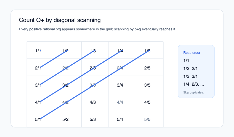
Figure. The diagonal scan turns a two-dimensional grid into one sequence; the lowest-terms condition removes duplicate names for the same rational.

Density is a different property. The rationals meet every nonempty open interval of the real line, but the diagonal procedure still places them in a single list. Dense does not mean uncountable.

Products of countable sets

The grid argument also gives a useful explicit pairing of two copies of $N$. For $a,b\in N$, let

$$\pi(a,b)=\frac{(a+b)(a+b+1)}2+b.$$

All pairs with fixed $a+b=s$ form a finite diagonal, and the triangular number $s(s+1)/2$ skips exactly the preceding diagonals. Therefore $\pi$ lists every pair once. More formally, from $n=\pi(a,b)$ one recovers the unique diagonal $s$ satisfying $s(s+1)/2\le n\lt (s+1)(s+2)/2$, then $b=n-s(s+1)/2$ and $a=s-b$. Thus $\pi:N\times N\to N$ is a bijection.

Theorem

A countable triple is countable

$|N\times N\times N|=|N|$.

Proof. Define

$$\Phi(a,b,c)=\pi(\pi(a,b),c).$$

Both applications of $\pi$ are bijections, so their composition is a bijection from $N^3$ to $N$. The inverse first recovers $(\pi(a,b),c)$ and then recovers $(a,b)$. This is the concrete content of “countable times countable times countable”: a finite-dimensional grid can be scanned by successive finite diagonals. The argument also handles empty factors in the usual way: if one factor is empty, the product is empty and therefore finite; the displayed bijection concerns three copies of $N$.

The same pairing handles a finite number of labelled copies of a countable set. For example, map $(n,0)$ and $(n,1)$ into $N$ by $(n,i)\mapsto\pi(n,i)$. The map is injective, so two copies of $N$ can be stored in one copy of $N$; applying the inverse pairing to the appropriate coordinates recovers the label and the original number. This explains why an infinite list can absorb a finite amount of extra bookkeeping. It does not say that every enlargement has the same size: the existence of the particular map must still be proved.

More generally, cardinality comparisons can be transported through maps. If $X\to Y$ and $Y\to Z$ are injections, their composition gives $|X|\le|Z|$. If both maps are bijections, the composition is a bijection. These two simple rules are the bookkeeping behind the integer, rational, and triple enumerations in this section.

Cardinal inequalities

Definition

Cardinal inequality

For sets $X$ and $Y$, write

$$|X|\le |Y|$$

if there exists an injection $X\to Y$. Write $|X|\lt|Y|$ if $|X|\le|Y|$ and $|X|\ne|Y|$.

The arrow direction is essential: an injection from $X$ into $Y$ says that $Y$ has enough distinct locations to store every element of $X$, so the domain is the no-larger side. The inclusion $N\to Z$, $n\mapsto n$, proves $|N|\le|Z|$; it does not alone prove equality. The enumeration of $Z$ supplies the reverse size comparison, or the explicit bijection above supplies equality directly.

Worked example

A finite comparison with unused codomain elements

The map $r:\{1,2,3\}\to\{a,b,c,d\}$ given by $r(1)=b$, $r(2)=d$, $r(3)=a$ is injective. Thus $|\{1,2,3\}|\le|\{a,b,c,d\}|$. It is not surjective because $c$ is unused, which is exactly why the inequality may be strict.

Theorem

Cardinal inequalities form a partial-order pattern

The relation $\le$ is reflexive, transitive, and antisymmetric on cardinalities. Consequently $\lt$ is irreflexive and transitive.

Proof. Reflexivity follows from the injective identity map $id_X:X\to X$. For transitivity, if $f:X\to Y$ and $g:Y\to Z$ are injections, then $g\circ f$ is injective: equality of its outputs first gives equality of the $f$ outputs, then equality of inputs. Antisymmetry is precisely the Cantor-Bernstein theorem below. Finally, $|X|\lt|X|$ is impossible because $|X|=|X|$; transitivity of strict inequality follows by combining transitivity of $\le$ with the unequal-cardinality conditions.

There is no set whose elements are all sets. Assuming such a universal set would permit a Russell-type self-membership construction and a contradiction. Accordingly, $\le$ is not being presented as one relation with a global “set of all sets” as its domain. The partial-order statements are about any chosen collection of sets, or the cardinalities represented by that collection, that we are comparing. This qualification is foundational bookkeeping; it does not change any of the maps or proofs above.

A surjection $X\to Y$ intuitively says that $Y$ is no larger than $X$, but turning that intuition into an injection $Y\to X$ requires selecting one preimage for each $y\in Y$. The next note examines that choice issue; here we use injections and bijections directly, without assuming a choice function.

Cantor-Bernstein: the two injections fit together

Theorem

Cantor-Bernstein theorem

If $f:X\to Y$ and $g:Y\to X$ are injections, then $|X|=|Y|$.

Using $f$ everywhere may leave elements of $Y$ uncovered; using $g^{-1}$ everywhere may fail because it is defined only on $g(Y)$. A point outside $g(Y)$ must therefore use $f$. Once a point $x$ uses $f$, the point $g(f(x))$ cannot use $g^{-1}$: the two branches would have the same output. The layers below propagate this requirement through repeated applications of $g\circ f$.

Start with

$$A_0=X,\qquad B_0=g(Y),$$

then define successive sets recursively, using the initial-value-and-successor pattern of 3.2 Induction and recursive arithmetic:

$$A_{n+1}=g(f(A_n)),\qquad B_{n+1}=g(f(B_n)).$$

Because $g(Y)\subseteq X$, these sets are nested:

$$A_0\supseteq B_0\supseteq A_1\supseteq B_1\supseteq A_2\supseteq B_2\supseteq\cdots.$$

The inclusions are inductive: $A_1\subseteq B_0$, then $B_{n+1}\subseteq A_{n+1}$, and the preceding inclusion $A_n\subseteq B_{n-1}$ gives $A_{n+1}\subseteq B_n$. If $X$ or $Y$ is empty, the two injections force both sets to be empty and the unique empty map is the required bijection; the construction below also covers that case.

The layer $A_n\setminus B_n$ is the part on which we will use $f$; the remaining points lie in $g(Y)$ and will use the inverse of $g$ on its image.

Proof. First note that $g\circ f:X\to X$ is injective. For every $n$, it maps $A_n\setminus B_n$ bijectively onto $A_{n+1}\setminus B_{n+1}$. Indeed, injectivity gives one-to-one behavior. If $z\in A_{n+1}\setminus B_{n+1}$, write $z=g(f(x))$ with $x\in A_n$; if $x\in B_n$, then $z\in g(f(B_n))=B_{n+1}$, a contradiction. Therefore $x\in A_n\setminus B_n$, proving onto behavior between the layers.

Define $h:X\to Y$ by

$$h(x)= \begin{cases} f(x),&x\in A_n\setminus B_n\text{ for some }n,\\ g^{-1}(x),&x\notin A_n\setminus B_n\text{ for every }n. \end{cases}$$

Here $g^{-1}$ means the inverse of the bijection $g:Y\to g(Y)$, not an inverse on all of $X$. The second case is defined: a point outside every layer cannot be in $A_0\setminus B_0=X\setminus g(Y)$, so it belongs to $g(Y)$. The layers are disjoint because they come from a nested sequence, so $h$ is well-defined.

To prove injectivity, suppose $h(x_1)=h(x_2)$. If both points lie in layers, injectivity of $f$ gives $x_1=x_2$. If both are in the second case, injectivity of $g^{-1}$ gives equality. In the mixed case, say $x_1\in A_n\setminus B_n$ and $h(x_2)=g^{-1}(x_2)$, the equality implies $x_2=g(f(x_1))$. The layer mapping just proved puts $x_2$ in $A_{n+1}\setminus B_{n+1}$, contradicting that $x_2$ was in the second case.

For surjectivity, take $y\in Y$ and put $x=g(y)\in X$. If $x$ is in no layer, then $h(x)=g^{-1}(x)=y$. Otherwise $x\in A_n\setminus B_n$. It cannot be in the zeroth layer, since $A_0\setminus B_0=X\setminus g(Y)$ while $x\in g(Y)$. Hence $n\ge1$; the layer bijection gives an $x'\in A_{n-1}\setminus B_{n-1}$ with $g(f(x'))=x=g(y)$. Since $g$ is injective, $f(x')=y$, and therefore $h(x')=y$. Thus $h$ is surjective and bijective, proving $|X|=|Y|$. No choice function is used: the construction is determined by the given $f$ and $g$.

Power sets and Cantor's theorem

Definition

Power set notation

For a set $X$, the notation $2^X$ denotes the set of all subsets of $X$.

Thus

$$T\in 2^X$$

means exactly that $T\subseteq X$.

The notation $2^X$ is suggestive: if $X$ has $n$ elements, then its power set has $2^n$ subsets. Cantor's theorem says that the power set is larger not only for finite sets, but for every set.

For the empty set this notation is already informative:

$$2^\varnothing=\{\varnothing\}.$$

There is one subset of the empty set, namely the empty set itself. Thus the finite pattern $|2^X| = 2^{|X|}$ starts with $2^0=1$. The theorem below is stronger than this finite counting rule: it compares cardinalities even when there is no finite number that counts the elements.

A subset missing from a proposed list

Suppose a function $f:X\to2^X$ assigns one subset to each element of $X$. To find a subset omitted by $f$, it is enough to make it differ from $f(x)$ at one element for each $x$. The index $x$ itself supplies that element: include $x$ precisely when $f(x)$ excludes it. Each row of the proposed list then has a specific reason to disagree with the constructed subset.

Here is a finite illustration with $X=\{a,b,c\}$. Each row records one proposed value of $f$; a $1$ means that the column element belongs to that subset, and a $0$ means that it does not. The bold entries in the first three rows lie on the diagonal.

Read the diagonal as $1,0,1$ and reverse each decision to obtain $0,1,0$. Thus $T=\{b\}$. It differs from $f(a)$ at $a$, from $f(b)$ at $b$, and from $f(c)$ at $c$. Agreement at other positions cannot repair even one of these differences.

For an arbitrary set, the same rule is $x\in T$ exactly when $x\notin f(x)$. It makes one membership decision for each element of $X$, without requiring a numerical ordering of $X$ or an infinite scanning procedure.

Cantor's theorem

Theorem

Cantor's theorem

Let $X$ be a set. Then

$$|X|\lt |2^X|.$$

The proof has two parts.

First, there is an injection

$$X\to 2^X,\qquad x\mapsto \{x\}.$$

So $|X|\le |2^X|$. For example, when $X=\{a,b\}$, this map selects two of the four subsets $\varnothing,\{a\},\{b\},\{a,b\}$; it need not hit every subset.

Second, there is no bijection from $X$ to $2^X$. Suppose, for contradiction, that $f:X\to 2^X$ were a bijection. Define the diagonal set

$$T=\{x\in X\mid x\notin f(x)\}.$$

Since $T$ is a subset of $X$, we have $T\in 2^X$. If $f$ were surjective, there would be some $y\in X$ such that

$$f(y)=T.$$

Now ask whether $y\in T$.

• If $y\in T$, then by definition of $T$, $y\notin f(y)=T$, a contradiction.
• If $y\notin T$, then by definition of $T$, $y\in f(y)=T$, again a contradiction.

Both cases are impossible. Therefore no bijection $X\to 2^X$ exists, and hence $|X|\lt |2^X|$.

When $X=\varnothing$, the power set has one element and no function from $X$ can hit it. Thus the same conclusion includes the empty-set case.

Proof X-Ray

Where surjectivity enters

The equation $f(y)=T$ is the decisive use of surjectivity. The diagonal argument does not use injectivity: it rules out every surjection from $X$ onto $2^X$. The singleton injection supplies the other part of the strict cardinal inequality.

The real numbers are uncountable

Theorem

The reals are uncountable

The set $R$ of real numbers is uncountable. In particular,

$$|N|\lt |R|.$$

The proof uses Cantor's theorem and an injection from $2^N$ into $R$.

By Cantor's theorem,

$$|N|\lt |2^N|.$$

So it is enough to show

$$|2^N|\le |R|.$$

Given a subset $S\subseteq N$, encode it by a sequence of zeros and ones:

$$a_n= \begin{cases} 1, & n\in S,\\ 0, & n\notin S. \end{cases}$$

Then define

$$\phi(S)=\sum_{n=0}^{\infty}\frac{a_n}{3^{n+1}}\in [0,1].$$

This sends each subset of $N$ to a real number.

Worked example

Encoding a subset of N

If

$$S=\{0,2,5,\ldots\},$$

then the beginning of the sequence is

$$a_0=1,\quad a_1=0,\quad a_2=1,\quad a_3=0,\quad a_4=0,\quad a_5=1.$$

The corresponding real number begins as

$$\phi(S)=\frac13+\frac1{3^3}+\frac1{3^6}+\cdots .$$

The partial sums are nondecreasing and bounded above by $1/2$, so completeness gives a real limit. This is the same passage from finite approximations to a real number used in 4.6 Decimal expansions and irrational numbers; no conversion to decimal notation is needed.

Why use base $3$ rather than base $2$? Base $3$ is useful so that distinct zero-one sequences cannot be cancelled by the tail.

If $S\ne S'$, let $k$ be the first index where the two associated sequences differ. At index $k$, the two sums differ by exactly

$$\frac1{3^{k+1}}.$$

The total possible contribution from all later terms is at most

$$\sum_{n=k+1}^{\infty}\frac1{3^{n+1}} =\frac1{2\cdot 3^{k+1}},$$

which is strictly smaller than the first differing contribution. Therefore the two real numbers are not equal. Hence $\phi$ is injective, and $|2^N|\le |R|$.

Combining this with Cantor's theorem gives

$$|N|\lt |2^N|\le |R|,$$

so $R$ is uncountable.

Common mistake

The proof only needs an injection into R

To prove $|2^N|\le |R|$, we do not need every real number to be hit by $\phi$. We only need distinct subsets of $N$ to produce distinct real numbers.

Worked example

A finite version of the ternary separation

Take two binary sequences which first differ at index $k=2$. The contribution at that index has size $1/27$. Even if every later binary digit favours the other sequence, the total later contribution is

$$\frac1{3^4}+\frac1{3^5}+\cdots=\frac1{54},$$

which is only half as large. Thus the first disagreement cannot be cancelled. The same geometric-series estimate works for any first differing index.

In the other direction, fix an enumeration $Q=\{q_1,q_2,\ldots\}$ and define

$$\rho(r)=\{n-1:n\ge1,\ q_n\lt r\}\subseteq\mathbb N.$$

This records the rationals below $r$ by their indices. The rational-density result in 4.4 Axioms for the reals and first approximations ensures that if $r\lt s$, some $q_n$ satisfies $r\lt q_n\lt s$. Hence $\rho(r)\ne\rho(s)$. Thus $\rho:R\hookrightarrow2^N$ is injective.

Identifying the continuum cardinal

Write $\mathcal P(\mathbb N)=2^{\mathbb N}$ for the set of all subsets of $\mathbb N$, and set $\mathfrak c=|\mathbb R|$. The zero–one ternary construction above is an injection $\mathcal P(\mathbb N)\hookrightarrow\mathbb R$, while the rational-index construction is an injection $\mathbb R\hookrightarrow\mathcal P(\mathbb N)$. Applying the proved Cantor–Bernstein theorem to these two specific maps gives

$$\mathfrak c=|\mathbb R|=|\mathcal P(\mathbb N)|=2^{\aleph_0}.$$

Here $2^{\aleph_0}$ denotes cardinal exponentiation: functions from $\mathbb N$ to $\{0,1\}$ correspond bijectively to subsets by their indicator functions. This equality does not assert $\mathfrak c=\aleph_1$; $\aleph_1$ is the least uncountable cardinal in the usual aleph ordering.

The continuum hypothesis

Hypothesis — Continuum hypothesis.

The continuum hypothesis says that there is no set $S$ such that

$$|N|\lt |S|\lt |R|.$$

This is a natural guess after seeing that $R$ is larger than $N$: perhaps there is no intermediate size between the countably infinite cardinality and the cardinality of the continuum.

This guess has a surprising formal status. The continuum hypothesis is independent of the usual axioms of set theory, ZFC. More precisely, if ZFC is consistent, then neither CH nor its negation is provable from ZFC: Godel's result gives the relative consistency of ZFC+CH, and Cohen's forcing result gives the relative consistency of $ZFC+\neg\mathrm{CH}$. These are metamathematical consistency results, not proofs of CH or of its negation inside this course.

For this course, the point is not to prove those metamathematical results but to recognize where axioms matter. Cantor's theorem and real uncountability remain ZFC theorems; CH asks for a sharper comparison between them. In later proofs, record map directions and mark any use of choice or maximality.

Thus “independent” does not mean that CH is meaningless or that every cardinal statement is undecidable. It means that the usual ZFC axioms do not settle this particular intermediate-size question; CH itself is an additional hypothesis.

Countable unions of countable sets

Theorem

A countable union of countable sets is countable

Assuming the axiom of choice, if ${A_n}_{n\in N}$ is a countable family of countable sets, then

$$A=\bigcup_{n\in N} A_n$$

is countable.

The empty-union case is immediate: if $A=\varnothing$, the empty function is an injection into $N$. Now assume $A$ is nonempty. Since each $A_n$ is countable, for each index $n$ there exists an injection

$$i_n:A_n\to N.$$

When $A_n=\varnothing$, the unique empty function is such an injection. We use the axiom of choice to choose the whole family of injections ${i_n}$ simultaneously, including those empty-member cases. This is a choice issue about the family of witnesses; it is not a claim that a countable union of arbitrary uncountable sets is countable.

Now define

$$h:A\to N\times N,\qquad h(x)=(n(x),i_{n(x)}(x)),$$

where

$$n(x)=\min\{n\in N\mid x\in A_n\}.$$

The index set is nonempty because $x$ belongs to the union, and the well-ordering of $N$ gives its least element. This consequence of induction is proved in 6.3 Intervals, Cantor set, density, and well-ordering. The map $h$ is injective. If $h(x)=h(x')$, equality of the first coordinates gives $n(x)=n(x')=n$. Equality of the second coordinates then gives $i_n(x)=i_n(x')$, and the injectivity of $i_n$ gives $x=x'$.

Finally, diagonal enumeration gives an injection $N\times N\to N$, so composing it with $h$ makes $A$ countable. List $(0,0)$, then the pairs whose coordinates sum to $1$, then those whose coordinates sum to $2$, and so on; each pair appears at a finite stage. The index set and every member must be countable: an uncountable index set of singletons, or one uncountable member, can make the union uncountable. Empty members contribute no element.

Common mistake

Countable union is not the same as arbitrary union

The theorem here is about a countable family ${A_n}$. It does not say that an arbitrary union of countable sets must be countable.

Work in the usual classical set-theoretic setting, including the axiom of choice for ordered aleph cardinals. Use the definitions and results on countability, Cantor’s theorem, cardinal comparison, and the continuum hypothesis developed in the preceding material.

Examples

Intervals have continuum size. The map $x\mapsto x/\sqrt{1+x^2}$ bijects $\mathbb R$ with $(-1,1)$; its inverse is $u\mapsto u/\sqrt{1-u^2}$. Direct substitution verifies both identities and the square-root domains. An affine map then bijects $(-1,1)$ with any nonempty bounded open interval. Thus a short interval has the same cardinality as the whole real line, without assuming CH.

Irrationals even have continuum size. Let $T=\{\sqrt2+n:n\in\mathbb Z\}$, a countably infinite set of irrational numbers. The union $\mathbb Q\cup T$ is countably infinite, so choose its enumeration and an enumeration of $T$ to obtain a bijection between them. Extend that bijection to $\mathbb R$ by fixing every point outside $\mathbb Q\cup T$. Its range is exactly the irrationals: the original rational points and $T$ are reassigned bijectively onto $T$, and every remaining irrational stays fixed. Thus $|\mathbb R\setminus\mathbb Q|=\mathfrak c$. This explicit countable reassignment is stronger than merely proving irrational uncountability, and still says nothing about all other uncountable subsets.

Density is unrelated to the missing cardinal gap. The rationals are dense and countable; the irrationals are dense and continuum-sized. Neither property forces a claim about every possible intermediate subset. Exhibiting many particular uncountable sets of size $\mathfrak c$ is not a proof of CH, whose quantifier concerns every potential intermediate size.

Exercises

P01. Statement. State CH using cardinal inequalities and in a sentence about infinite subsets of $\mathbb R$. Explain the role of $\aleph_1$.

P02. Required proof. Prove the irrationals are uncountable using only real uncountability and rational countability. Identify the invalid step in “irrationals are dense, therefore uncountable.”

P03. Inverse verification. Check both compositions for $x/\sqrt{1+x^2}$ and its stated inverse, including signs of square roots.

P04. Proof audit. A student argues “the reals are uncountable and $\aleph_1$ is uncountable, so their cardinalities agree.” Explain the missing comparison.

P05. Injection versus bijection. Explain why the map $r\mapsto\{q\in\mathbb Q:q<r\}$ is injective, and why that fact alone does not prove $\mathfrak c=2^{\aleph_0}$. Name the additional ingredients supplied above.

P06. Consequence distinction. Decide which follow without assuming CH: rational countability; real uncountability; irrational continuum size; every uncountable subset of $\mathbb R$ having continuum size. Justify each classification without claiming to prove or disprove CH.

Full solutions

P01. CH is the assertion that no cardinal lies strictly between $\aleph_0$ and $\mathfrak c$, equivalently no infinite subset of $\mathbb R$ is both uncountable and smaller than the continuum. In the usual aleph ordering, $\aleph_1$ is the least uncountable cardinal, so CH is $\mathfrak c=\aleph_1$. The symbol is defined independently of whether that equality holds.

P02. If both $\mathbb Q$ and its real complement were countable, their union would be countable, contradicting real uncountability. Density alone does not imply uncountability because $\mathbb Q$ itself is a dense countable counterexample.

P03. For $u=x/\sqrt{1+x^2}$, $1-u^2=1/(1+x^2)>0$, whose positive square root is $1/\sqrt{1+x^2}$. Therefore $u/\sqrt{1-u^2}=x$. Conversely for $|u|<1$, setting $x=u/\sqrt{1-u^2}$ gives $1+x^2=1/(1-u^2)$, so $x/\sqrt{1+x^2}=u$. Both inverses are valid for negative as well as positive inputs because each denominator square root is positive.

P04. Uncountable is not a single cardinal value; it merely excludes countable sizes. Minimality of $\aleph_1$ proves $\aleph_1\le\mathfrak c$. The reverse inequality or a bijection is missing, and its equality conclusion is precisely CH rather than an automatic inference.

P05. For $r<s$, choose rational $q$ with $r<q<s$. It lies below $s$ but not below $r$, so the assigned subsets differ. This gives only an injection from reals into a rational power set. The reverse injection from subsets of the natural numbers (encoded by 0–1 indicator sequences) to ternary real numbers using digits 0 and 1, the enumeration-induced equivalence of the two power sets, and Cantor–Schroeder–Bernstein together establish equality.

P06. The first three follow from the explicit enumeration, diagonal and countable-reassignment arguments in the preceding canonical material and examples, without CH. The final universal assertion is an equivalent formulation of CH in the stated setting, so it is not obtained from those earlier proofs. The distinction is between specific constructed bijections and a claim ruling out every possible intermediate-size subset.