Column space, row space, and rank

Proof of the finite real matrix product laws

Let $m,n,p,q$ be positive integers, let $A\in\mathbb R^{m\times n}$, $B\in\mathbb R^{n\times p}$, and $C\in\mathbb R^{p\times q}$. All the following arguments use the row-by-column definition and finite real sums. For any output position $(i,\ell)$,

$$\begin{aligned} ((AB)C)_{i\ell} &=\sum_{k=1}^{p}\left(\sum_{j=1}^{n}a_{ij}b_{jk}\right)c_{k\ell}\\ &=\sum_{j=1}^{n}a_{ij}\left(\sum_{k=1}^{p}b_{jk}c_{k\ell}\right) =(A(BC))_{i\ell}. \end{aligned}$$

The middle equality only reorders two finite sums and uses real distributivity. Both products are $m\times q$, so equality at every position proves associativity. No factor has changed its order.

For $D\in\mathbb R^{n\times p}$, the same definition gives

$$[A(B+D)]_{ik}=\sum_{j=1}^{n}a_{ij}(b_{jk}+d_{jk}) =(AB)_{ik}+(AD)_{ik}.$$

For $E\in\mathbb R^{m\times n}$, it gives

$$[(A+E)B]_{ik}=\sum_{j=1}^{n}(a_{ij}+e_{ij})b_{jk} =(AB)_{ik}+(EB)_{ik}.$$

Thus both distributive laws hold with the displayed matching sizes. For every real scalar $c$,

$$[(cA)B]_{ik}=\sum_j(ca_{ij})b_{jk} =c\sum_j a_{ij}b_{jk} =\sum_j a_{ij}(cb_{jk})=[A(cB)]_{ik},$$

proving $(cA)B=c(AB)=A(cB)$ by entrywise equality. In particular, for $x,y\in\mathbb R^n$ and real $s,t$,

$$[A(sx+ty)]_i=\sum_j a_{ij}(sx_j+ty_j) =s(Ax)_i+t(Ay)_i.$$

This proves the matrix-vector linearity used when comparing solutions of the same linear system. All identities concern compatible finite real matrices; they do not assert commutativity or cancellation of arbitrary matrix factors.

Build the elementary matrix from the identity

Suppose an elementary row operation $\rho$ is meant to act on matrices with $p$ rows. Start with the identity matrix $I_p$, apply the same elementary row operation to $I_p$, and call the result $E_\rho$. All scalars are taken from the underlying field of the matrices; in particular, every nonzero scaling factor $c$ has a reciprocal $1/c$ in that field.

Definition

Elementary row-operation matrix

The elementary row-operation matrix associated with an elementary row operation $\rho$ on $p$-row matrices is the $p \times p$ matrix obtained by applying $\rho$ to $I_p$.

This matrix is also called an elementary matrix. The longer name keeps its connection with the specified row operation visible.

Equivalently,

$$E_\rho = \rho(I_p).$$

The reason this definition is useful is the following theorem.

Theorem

Elementary row operations are left multiplication

Let $A$ be any matrix with $p$ rows. If $\rho$ is one elementary row operation and $\rho(A)$ denotes the result of applying it to $A$, then

$$\rho(A) = E_\rho A.$$

So applying that elementary row operation to $A$ is the same as multiplying $A$ on the left by the elementary row-operation matrix obtained from the same operation on $I_p$.

The multiplication must be on the left. Row operations change rows by mixing rows. Left multiplication forms new rows of $A$ as linear combinations of old rows of $A$. Right multiplication would instead mix columns.

The dimensions make the same point. If $A$ is $p \times n$, then $E_\rho$ is $p \times p$, so $E_\rho A$ is defined and remains $p \times n$. There is no assumption that $A$ is square. By contrast, a column-operation matrix acting on these same $n$ columns would have size $n \times n$ and multiply on the right.

Why left multiplication performs the operation

Proof

Verify the three elementary cases row by row

Write the rows of an arbitrary $p \times n$ matrix $A$ as $a_1,a_2,\ldots,a_p$, and let $e_k^{\mathsf T}$ denote row $k$ of $I_p$. The basic identity

$$e_k^{\mathsf T}A=a_k$$

says that a row of a left multiplier selects the corresponding row of $A$. Now check the three elementary operations.

1. For $R_i\leftrightarrow R_j$, the matrix $E_\rho$ has row $i$ equal to $e_j^{\mathsf T}$, row $j$ equal to $e_i^{\mathsf T}$, and every other row $k$ equal to $e_k^{\mathsf T}$. Thus the rows of $E_\rho A$ are the rows of $A$ with precisely rows $i$ and $j$ exchanged.

2. For $R_i\leftarrow cR_i$, where $c\ne0$, row $i$ of $E_\rho$ is $c e_i^{\mathsf T}$ and all other rows are unchanged. Hence row $i$ of the product is

   $$(c e_i^{\mathsf T})A=c a_i,$$

   while row $k$ remains $a_k$ for $k\ne i$.

3. For $R_j\leftarrow R_j+cR_i$, where $i\ne j$, row $j$ of $E_\rho$ is $e_j^{\mathsf T}+c e_i^{\mathsf T}$ and every other row is unchanged. Therefore the new row $j$ is

   $$(e_j^{\mathsf T}+c e_i^{\mathsf T})A=a_j+c a_i,$$

   exactly as prescribed.

These cases exhaust the elementary row operations, so they prove $E_\rho A=\rho(A)$ for every compatible $A$. The proof does not claim that an arbitrary manipulation of rows has such an elementary matrix; $\rho$ must be one of the three operations just checked.

Acting on an augmented matrix

Suppose $Ax=b$ is represented by the augmented matrix $[A\mid b]$. An elementary row operation must act on the full augmented matrix, not separately on whichever entries happen to be convenient. The multiplication identity is

$$E_\rho[A\mid b]=[E_\rho A\mid E_\rho b].$$

Thus the coefficients and the right-hand side undergo the same combination of rows. A vector $x$ satisfies $Ax=b$ if and only if it satisfies $E_\rho Ax=E_\rho b$: the forward implication follows by multiplying the equation by $E_\rho$, and the reverse implication follows by applying the reverse elementary operation. This is the precise reason the solution set is preserved.

Changing only $A$ while leaving $b$ fixed, or changing only $b$, generally produces a different system. The augmentation bar is therefore a visual separator, not a boundary at which a row operation may stop.

A sequence of elementary row operations becomes one matrix product

The real payoff is not just representing one elementary row operation. A whole sequence of elementary row operations becomes one product of elementary row-operation matrices.

Theorem

A sequence of elementary row operations as a product

Suppose

$$A_1 \xrightarrow{\rho_1} A_2 \xrightarrow{\rho_2} A_3 \xrightarrow{\rho_3} \cdots \xrightarrow{\rho_k} A_{k+1}.$$

Then

$$A_{k+1} = E_{\rho_k}E_{\rho_{k-1}}\cdots E_{\rho_2}E_{\rho_1}A_1.$$

Here every $\rho_j$ is an elementary row operation on matrices with the same number of rows. The product represents the whole sequence, although the product itself need not be a single elementary row-operation matrix.

The order in this formula is important. The first row operation appears closest to $A_1$, because it is applied first:

$$A_2 = E_{\rho_1}A_1, \qquad A_3 = E_{\rho_2}A_2 = E_{\rho_2}E_{\rho_1}A_1.$$

Worked example

Two row operations combined

Let

$$A = \begin{bmatrix} 1 & 0 & 1\\ 0 & 2 & 1\\ 1 & 0 & 0 \end{bmatrix}.$$

Apply

$$\rho_1:\ R_2 \leftarrow R_2 + R_1, \qquad \rho_2:\ R_1 \leftarrow R_1 + 2R_2.$$

The corresponding row-operation matrices are

$$E_{\rho_1} = \begin{bmatrix} 1 & 0 & 0\\ 1 & 1 & 0\\ 0 & 0 & 1 \end{bmatrix}, \qquad E_{\rho_2} = \begin{bmatrix} 1 & 2 & 0\\ 0 & 1 & 0\\ 0 & 0 & 1 \end{bmatrix}.$$

After both operations, the result is

$$E_{\rho_2}E_{\rho_1}A = \begin{bmatrix} 3&2&0\\ 1&1&0\\ 0&0&1 \end{bmatrix} \begin{bmatrix} 1&0&1\\ 0&2&1\\ 1&0&0 \end{bmatrix} = \begin{bmatrix} 3&4&5\\ 1&2&2\\ 1&0&0 \end{bmatrix}.$$

Instead of multiplying $E_{\rho_2}E_{\rho_1}$ directly, you can also obtain this combined matrix by applying the same two elementary row operations to $I_3$ in the same order. The final numerical matrix also confirms that the second operation uses the already-updated row $2$.

Reverse row operations and inverses

Every elementary row operation has a reverse operation:

• the reverse of $R_j \leftarrow R_j + cR_i$ is $R_j \leftarrow R_j - cR_i$;
• the reverse of $R_i \leftarrow cR_i$, with $c \ne 0$, is $R_i \leftarrow (1/c)R_i$;
• the reverse of a row swap is the same row swap.

This gives a precise matrix statement.

Theorem

Elementary row-operation matrices are invertible

Every elementary row-operation matrix is invertible. Its inverse is the elementary row-operation matrix corresponding to the reverse elementary row operation.

Proof

Why the reverse matrix is a two-sided inverse

Let $E_\rho$ represent an elementary row operation $\rho$, and let $E_{\rho^{-1}}$ represent the reverse elementary operation. For every matrix $X$ with $p$ rows, applying $\rho$ and then reversing it restores $X$. By the left-multiplication theorem,

$$E_{\rho^{-1}}E_\rho X=X.$$

This statement holds for every such $X$; in particular, put $X=I_p$ to obtain $E_{\rho^{-1}}E_\rho=I_p$. Reversing first and then applying $\rho$ similarly gives $E_\rho E_{\rho^{-1}}=I_p$. Hence

$$E_\rho^{-1}=E_{\rho^{-1}}.$$

Concretely, a swap is its own inverse, scaling by $c\ne0$ is undone by scaling by $1/c$, and adding $c$ times row $i$ to row $j$ is undone by adding $-c$ times row $i$ to row $j$.

For example, if

$$E = \begin{bmatrix} 1 & 0 & 0\\ 3 & 1 & 0\\ 0 & 0 & 1 \end{bmatrix}$$

performs $R_2 \leftarrow R_2 + 3R_1$, then

$$E^{-1} = \begin{bmatrix} 1 & 0 & 0\\ -3 & 1 & 0\\ 0 & 0 & 1 \end{bmatrix}$$

performs $R_2 \leftarrow R_2 - 3R_1$.

This is the algebraic reason elementary row operations are reversible, and it explains why row reduction is so closely connected to invertible matrices.

Proof

Undo the last operation first

Let $E_1,\ldots,E_k$ encode a chronological chain on matrices with $p$ rows, so its combined multiplier is $J=E_k\cdots E_1$. Each inverse $E_j^{-1}$ represents the reverse of the corresponding elementary operation. To recover the input, the first move must undo $E_k$, because that was the last change made to the rows. The remaining reverse moves undo $E_{k-1},\ldots,E_1$ in that order. Consequently the reverse multiplier is

$$K=E_1^{-1}E_2^{-1}\cdots E_k^{-1}.$$

There are two orders to distinguish: the time order of the reverse operations starts with $E_k^{-1}$, while the written product places that first action nearest the matrix being restored. For three steps, associativity gives

$$KJ=E_1^{-1}E_2^{-1}(E_3^{-1}E_3)E_2E_1 =E_1^{-1}(E_2^{-1}E_2)E_1=I_p.$$

The other product $JK$ cancels adjacent inverse pairs starting with $E_1E_1^{-1}$ and also equals $I_p$. The same successive cancellation works for any finite chain. No factors have been commuted, and the argument does not require the matrix being transformed to be square.

Apply this reading to the earlier two-operation example. Its combined multiplier is $E_{\rho_2}E_{\rho_1}$, so its inverse is $E_{\rho_1}^{-1}E_{\rho_2}^{-1}$. Starting from the final matrix, first subtract twice the current second row from the first, recovering $[1\ 0\ 1]$ as the first row. Then subtract that recovered first row from the second, recovering $[0\ 2\ 1]$. Reversing the chain means restoring the intermediate states, which explains the order without a memorized rule.

Finite elimination terminates and preserves the solution set

Let $A\in\mathbb R^{m\times n}$, $b\in\mathbb R^m$, with positive finite integers $m,n$. The permitted row operations are an exchange of two distinct rows, multiplication of a row by a nonzero scalar, and addition of a scalar multiple of one row to a different row. Their inverses are respectively the same exchange, multiplication by the reciprocal, and subtraction of that multiple. Applying an operation to the entire augmented array therefore preserves exactly the solutions of $Ax=b$: the new equations are consequences of the old, and its inverse gives the reverse implication. Each operation is also multiplication on the left by the result of applying it to the identity matrix, an invertible elementary matrix.

Scan the coefficient columns from left to right, maintaining the next unused row. If the current column has a nonzero entry in an unused row, exchange that row into the next position, divide by its nonzero pivot, and subtract multiples of it from every other row to clear that column. Advance the unused-row index. If every unused entry in the column is zero, skip the column. Previously chosen pivot columns remain unit columns: the current unused rows have zeros in them, so the new pivot row and every subsequent subtraction preserve those zeros and earlier pivots. There are only $n$ column scans and at most $\min(m,n)$ pivots, each with finitely many row operations. Thus the algorithm terminates. At its end, the nonzero coefficient rows have increasing pivot columns and zeros below and above each pivot; any remaining coefficient row is zero. This proves the reduced echelon form used below, without assuming it will eventually appear.

Classification and the homogeneous freedom

Write $r$ for the number of pivots in the coefficient part. A zero coefficient row with a nonzero transformed right side is the impossible equation $0=c$, so the system has no solution. Otherwise assign arbitrary real values to all $n-r$ nonpivot variables. In each pivot row, its pivot variable equals the transformed right side minus the displayed linear combination of these free variables; no other pivot variable occurs. These formulas both construct a solution and recover every solution. If $r=n$ the solution is unique. If $r<n$, changing a free variable changes the vector, giving infinitely many solutions.

For $Az=0$ the free variables can all be zero, giving the zero solution. If $r<n$, set one free variable to one and the others to zero, and use the pivot formulas. This constructs a nonzero homogeneous solution. If $r=n$, the formulas force every homogeneous variable to zero. For a consistent system, fixing one solution $x_p$, subtraction proves that every solution has the form $x_p+z$ with $Az=0$, and substitution proves the converse.

For square $A$, if every column has a pivot, the coefficient form is $I$. The product $E$ of the finitely many elementary matrices satisfies $EA=I$. Since $E$ is invertible, $A=E^{-1}$ and therefore also $AE=I$: $E$ is a two-sided inverse. If a pivot is missing, the nonzero homogeneous solution constructed above rules out any inverse. This also justifies applying the same row operations to $[A\mid I]$ to obtain $[I\mid A^{-1}]$ in the invertible case.

Finite basis existence and extension, without a counting assumption

Let $V$ be a real vector space supplied with a finite spanning list $t_1,\ldots,t_N$. First prove that every independent list $u_1,\ldots,u_k$ has length at most $N$. After $j$ insertions, maintain a spanning list consisting of $u_1,\ldots,u_j$ and $N-j$ surviving old vectors. Expand $u_{j+1}$ in this list. Some coefficient on a surviving old vector is nonzero; otherwise $u_{j+1}$ would be in the span of the earlier $u_i$, contradicting independence. Solve for that old vector and replace it by $u_{j+1}$. The new list spans the same space and keeps every earlier insertion. If $k>N$, after $N$ steps the first $N$ independent vectors already span $V$, contradicting independence of $u_{N+1}$. This proves the bound, including $N=0$.

Every subspace $W$ has a finite basis. Start with the empty independent list. If its current span is not $W$, choose one vector of $W$ outside that span. A relation with nonzero coefficient on the new vector would express it in the old span, so the enlarged list remains independent. The proved bound permits at most $N$ additions; therefore the process stops with an independent spanning list for $W$. If $W=\{0\}$, it stops immediately with the empty basis. Starting instead with any given independent list in $W$ proves that list extends to a basis of $W$. Only a bounded finite selection is used. Finally, if two bases have sizes $p,q$, use each as the finite spanning list in the bound to obtain $p\le q$ and $q\le p$. Thus basis size, called dimension, is well-defined. This supplies the existence, extension and dimension facts used in rank–nullity.

A fixed matrix determines two subspaces:

• the subspace generated by its columns;
• the subspace generated by its rows.

They describe which outputs the matrix can produce and which linear equations its rows generate.

• Which right-hand sides $b$ can occur in a system $Ax = b$?
• How much independent linear information is actually stored in the rows?
• How many genuinely independent directions remain after all redundancy is removed?

The answers are called the column space, the row space, and the rank of the matrix.

Column space: what outputs can the matrix produce?

Let $A$ be an $m \times n$ matrix, and write its columns as

$$A = \begin{bmatrix} a_1 & a_2 & \cdots & a_n \end{bmatrix}.$$

Definition

Column space

The column space of $A$, written $C(A)$, is the span of the columns of $A$:

$$C(A) = \operatorname{Span}\{a_1, a_2, \ldots, a_n\}.$$

It is a subspace of $R^m$.

The most useful way to read this definition is through matrix multiplication. If $x = (x_1, \ldots, x_n)^t$, then

$$Ax = x_1 a_1 + x_2 a_2 + \cdots + x_n a_n.$$

So every vector of the form $Ax$ is a linear combination of the columns. Conversely, every linear combination of the columns can be written as $Ax$ for some vector $x$.

Theorem

Column space as an output set

For an $m \times n$ matrix $A$,

$$C(A) = \{Ax : x \in R^n\}.$$

Therefore a vector $b \in R^m$ belongs to $C(A)$ exactly when the system $Ax = b$ is consistent.

Row space: what linear information do the rows carry?

Write the rows of $A$ as $r_1,\ldots,r_m$, each a $1\times n$ matrix. To regard their span as a subspace of the usual column-vector space $\mathbb R^n$, we take their transposes explicitly.

Definition

Row space

The row space of $A$ is

$$R(A)=\operatorname{Span}\{r_1^T,\ldots,r_m^T\}=C(A^T) =\{A^Ts:s\in\mathbb R^m\}.$$

It is a subspace of $\mathbb R^n$.

Thus $x\in R(A)$ means $x=A^Ts$ for some $s\in\mathbb R^m$, or, equivalently, $x^T=s^TA$: the row $x^T$ is a linear combination of the rows of $A$. We may display rows horizontally while computing, but a row-space basis below consists of their transposes. This convention makes $R(A)=C(A^T)$ an actual equality of sets of column vectors.

The dimensions of the ambient spaces must be checked before comparing spaces. Columns of $A$ have $m$ entries, so $C(A)\subseteq\mathbb R^m$; transposed rows have $n$ entries, so $R(A)\subseteq\mathbb R^n$. Applying the same definition to $A^T$ also gives $C(A)=R(A^T)$. Even when $m=n$, having the same ambient space does not force equality of the two spans. The distinction concerns their members, not merely their names.

Rank counts the independent directions

The dimension of the column space is called the column rank. The dimension of the row space is called the row rank. One of the central theorems of linear algebra says that these numbers are equal.

Definition

Rank

The rank of a matrix $A$ is the number $r$ of pivots in its RREF. The basis theorem proved below will establish the equivalent dimension formula:

$$\operatorname{rank}(A) = \dim C(A) = \dim R(A).$$

When you row-reduce a matrix to RREF, the number of pivot columns is exactly the rank. So rank measures how many independent directions survive after all redundancy has been removed.

The pivot positions are read from the RREF, but the column-space basis vectors must be taken from the original matrix.

Worked example: read everything from one row reduction

Worked example

Column space, row space, and rank from a single matrix

Consider

$$A = \begin{bmatrix} 1 & 2 & 1 & 3 \\ 0 & 1 & 1 & 1 \\ 1 & 3 & 2 & 4 \end{bmatrix}.$$

Row-reducing gives

$$A \sim \begin{bmatrix} 1 & 0 & -1 & 1 \\ 0 & 1 & 1 & 1 \\ 0 & 0 & 0 & 0 \end{bmatrix} = R.$$

One explicit reduction is $R_3\leftarrow R_3-R_1$, followed by $R_3\leftarrow R_3-R_2$ and $R_1\leftarrow R_1-2R_2$. The third row becomes zero and the first two rows have their leading ones in columns one and two. This produces the displayed RREF rather than merely an echelon matrix with unexplained pivot positions.

There are two pivot columns, namely columns $1$ and $2$.

Write the columns of $A$ as

$$c_1 = \begin{bmatrix} 1 \\ 0 \\ 1 \end{bmatrix}, \quad c_2 = \begin{bmatrix} 2 \\ 1 \\ 3 \end{bmatrix}, \quad c_3 = \begin{bmatrix} 1 \\ 1 \\ 2 \end{bmatrix}, \quad c_4 = \begin{bmatrix} 3 \\ 1 \\ 4 \end{bmatrix}.$$

Then a basis for the column space is

$$\{c_1, c_2\}.$$

Indeed, the non-pivot columns are combinations of the pivot columns:

$$c_3 = -c_1 + c_2, \qquad c_4 = c_1 + c_2.$$

For the row space, we transpose the nonzero rows of $R$:

$$\{(1, 0, -1, 1)^T, (0, 1, 1, 1)^T\}.$$

So

$$\dim C(A) = 2, \qquad \dim R(A) = 2, \qquad \operatorname{rank}(A) = 2.$$

Finally, if

$$b = \begin{bmatrix} 5 \\ 2 \\ 7 \end{bmatrix},$$

then $b \in C(A)$ because

$$b = c_1 + 2c_2.$$

Equivalently, the system $Ax = b$ is consistent.

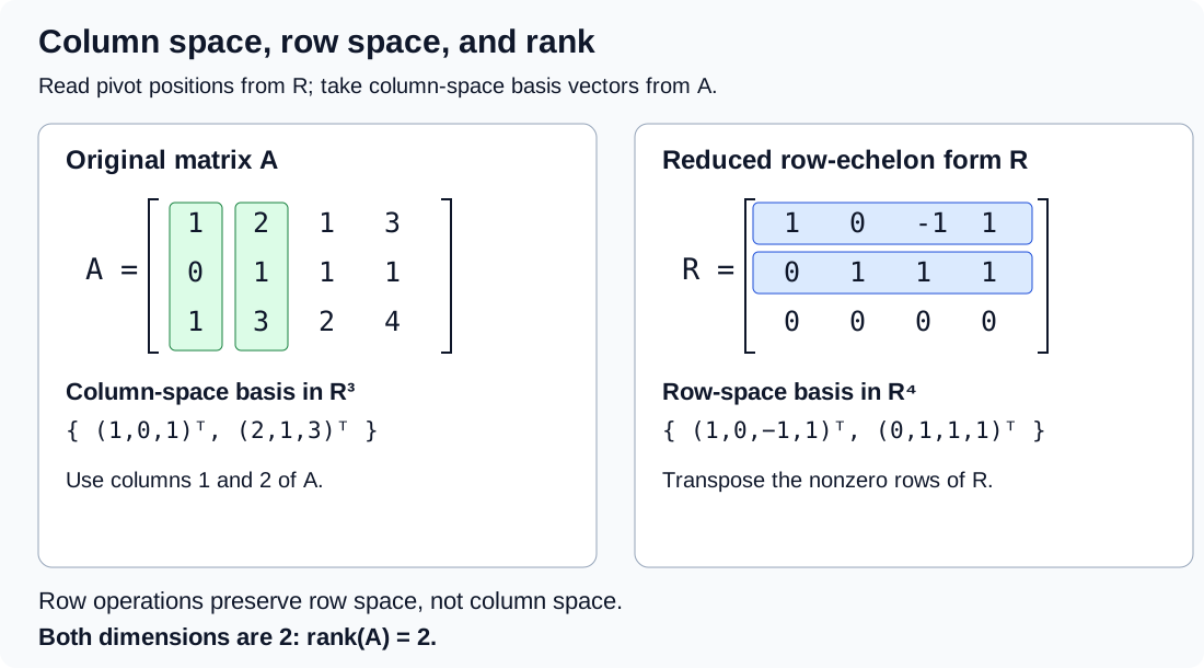
Static map for the worked example: pivot positions are read from the RREF, column-space basis vectors come from the original matrix, transposed nonzero RREF rows form a row-space basis, and both dimensions equal the rank.

Three results from one RREF

The following sequence revisits the same example. Distinguish the information read from the RREF from the column-space basis vectors taken from the original matrix.

Row reduction: what changes and what does not?

Row reduction preserves some of this structure while changing other parts.

Theorem

What invertible multiplication preserves

Let $A$ be a real $m\times n$ matrix, $G$ an invertible $n\times n$ matrix, and $H$ an invertible $m\times m$ matrix. Then

$$C(AG)=C(A),\qquad R(HA)=R(A).$$

In particular, row-equivalent matrices have the same row space. Their column spaces need not be equal.

Proof

Use the inverse for the reverse inclusion

If $y\in C(AG)$, write $y=AGs=A(Gs)$, so $y\in C(A)$. Conversely, if $y=At\in C(A)$, set $s=G^{-1}t$. Then $AGs=AGG^{-1}t=At=y$, giving the reverse inclusion. The first direction needs no inverse; the second uses it to produce a coefficient vector.

Now $(HA)^T=A^TH^T$, and $H^T$ is invertible with inverse $(H^{-1})^T$. Apply the just-proved result to get $R(HA)=C(A^TH^T)=C(A^T)=R(A)$. A sequence of row operations is left multiplication by an invertible $H$, so the row-equivalence assertion follows. Equivalently, every new row is a combination of old rows, and reversing the operations gives the other containment of their spans.

Left multiplication has a different effect on outputs: $C(HA)=\{Hy:y\in C(A)\}$. Indeed, $(HA)x=H(Ax)$ in both descriptions. This is an invertible image of the old column space, not necessarily the same subset of $\mathbb R^m$. If $A,B$ have the same number of rows, applying the same invertible $H$ gives $C(A)=C(B)$ if and only if $C(HA)=C(HB)$: the forward direction applies $H$ to equal sets, and the reverse applies $H^{-1}$. Comparing two transformed spaces is different from claiming that either one is unchanged.

Why the basis rules and rank equality hold

Theorem

Pivot bases and the equality of ranks

Let $Q$ be the RREF of a real $m\times n$ matrix $A$, with $r$ pivots in columns $j_1,\ldots,j_r$. The original columns $a_{j_1},\ldots,a_{j_r}$ form a basis of $C(A)$, and the transposes of the $r$ nonzero rows of $Q$ form a basis of $R(A)$. Consequently,

$$\dim C(A)=r=\dim R(A)=\operatorname{rank}(A).$$

Proof

Preserve coefficients and then inspect pivot coordinates

Write $Q=HA$ with $H$ invertible, and denote the columns of $Q$ by $q_j$. For every coefficient vector $c\in\mathbb R^n$,

$$\sum_{j=1}^n c_jq_j=H\left(\sum_{j=1}^n c_ja_j\right).$$

The left side is zero exactly when the sum inside parentheses is zero: one direction multiplies by $H$, the other by $H^{-1}$. Thus all homogeneous column relations, with their exact coefficients, are preserved in both directions. Relations involving only selected columns are covered by inserting zero coefficients in the remaining positions.

The pivot columns of $Q$ have a single one in distinct pivot rows and zeros elsewhere, so they are independent. Every column $q_j$ is their combination with coefficients $Q_{1j},\ldots,Q_{rj}$; all rows below $r$ are zero. The preserved relations show that the corresponding original pivot columns span every $a_j$. A zero combination of those original columns gives a zero combination of the pivot columns of $Q$, forcing every coefficient to vanish. This proves both spanning and independence for the column basis.

For the row basis, we already know $R(Q)=R(A)$. Deleting the zero rows leaves a spanning list of transposed nonzero rows. If their combination with coefficients $d_1,\ldots,d_r$ is zero, inspect coordinate $j_i$. In the RREF, that pivot column has one in row $i$ and zero in every other row, so this coordinate is exactly $d_i$. Hence all coefficients are zero and the list is independent. Each basis has $r$ members, proving the dimension equalities. When $r=0$, the matrix is zero, both spaces are the zero subspace in their respective ambient spaces, and both bases are empty.

This argument explains precisely why the reduction gives positions for the column basis but actual vectors for the row basis. It also yields $\operatorname{rank}(A^T)=\operatorname{rank}(A)$ by exchanging the two spaces. For an $m\times n$ matrix the rank is at most $\min(m,n)$, since the pivots occupy distinct rows and distinct columns. Rank is a number; no equality of row and column spaces is asserted by these equalities of numbers.

Equal dimensions do not identify the spaces

Worked example

Different spaces for one square matrix

Consider

$$D=\begin{bmatrix}1&0&0&1\\0&2&0&1\\0&0&3&1\\0&0&0&0\end{bmatrix}.$$

Its first three columns are independent: their first three coordinates force all coefficients of a zero combination to vanish. The fourth column is the first plus half the second plus one third the third. Consequently, $C(D)=\{(a,b,c,0)^T:a,b,c\in\mathbb R\}$ and its dimension is three. Both containment directions are explicit: every column has last coordinate zero, and any displayed vector is the combination of the first three columns with coefficients $a,b/2,c/3$.

The nonzero transposed rows are $(1,0,0,1)^T$, $(0,2,0,1)^T$ and $(0,0,3,1)^T$. They are independent by their first three coordinates, and the remaining row is zero, so they form a basis of $R(D)$. Their general combination shows

$$R(D)=\{(a,b,c,a+b/2+c/3)^T:a,b,c\in\mathbb R\}.$$

Thus $(1,0,0,1)^T\in R(D)$ but it is not in $C(D)$. Conversely, $(1,0,0,0)^T\in C(D)$ does not satisfy the displayed row-space condition. The two spaces are distinct subspaces of the same $\mathbb R^4$, although both have dimension three. Scaling the second and third rows by $1/2$ and $1/3$ gives three pivots, agreeing with rank three.

Counterexample mode

Row reduction can move the column space

False claim. Row-equivalent matrices have the same column space.

Take

$$A_0=\begin{bmatrix}1&0\\1&0\end{bmatrix},\qquad H=\begin{bmatrix}1&0\\-1&1\end{bmatrix},\qquad B_0=HA_0=\begin{bmatrix}1&0\\0&0\end{bmatrix}.$$

The operation is subtracting row one from row two, and adding it back supplies the inverse. Directly, $C(A_0)=\operatorname{Span}\{(1,1)^T\}$ whereas $C(B_0)=\operatorname{Span}\{(1,0)^T\}$. The nonzero vector $(1,0)^T$ cannot equal $t(1,1)^T$: its first coordinate would force $t=1$ and its second would force $t=0$. So the spaces differ. Yet both row spaces equal $\operatorname{Span}\{(1,0)^T\}$ and both ranks are one. Even the redundant second-column relation is preserved: it is zero in both matrices.

Repaired statement. Row operations preserve row space, rank and the coefficients of column relations. The actual column space becomes $C(HA)=\{Hy:y\in C(A)\}$; a basis for the original column space must use original columns at the pivot positions. In this example the RREF pivot column is not even a member of the original column space, so it cannot be its basis.

Test membership by keeping the right-hand side

Worked example

A column space described by one equation

Let

$$M=\begin{bmatrix}3&2&1&-4\\-1&1&-2&3\\2&-4&6&-8\end{bmatrix}.$$

Twice the first row plus sixteen times the second plus five times the third is zero. Hence every output $b=Mx$ satisfies $2b_1+16b_2+5b_3=0$. This proves one inclusion in the proposed description of $C(M)$; a condition satisfied by every output need not alone prove it describes every output.

For the converse, suppose this equation holds. Use only the first two columns, with coefficients

$$s=\frac{b_1-2b_2}{5},\qquad t=\frac{b_1+3b_2}{5}.$$

Their combination is $(3s+2t,-s+t,2s-4t)^T$. The first two coordinates are $b_1,b_2$, and the last is $(-2b_1-16b_2)/5=b_3$ by the assumed equation. Thus $M(s,t,0,0)^T=b$, proving the other inclusion. We obtain

$$C(M)=\{b\in\mathbb R^3:2b_1+16b_2+5b_3=0\} =N\!\left(\begin{bmatrix}2&16&5\end{bmatrix}\right).$$

For $v=(18,-6,12)^T$, the condition gives $36-96+60=0$; indeed $v$ is six times the first column. For $w=(2,1,-3)^T$, it gives $4+16-15=5\ne0$, so $Mx=w$ is inconsistent. One vector is accepted by an explicit coefficient choice, the other rejected by a necessary output equation.

More generally, if $Q=HA$ is an RREF with $r$ pivots, then $Ax=b$ is equivalent to $Qx=Hb$. Its zero rows require the last $m-r$ coordinates of $Hb$ to vanish; its pivot equations impose no further condition on the right-hand side. Taking these last rows of $H$ as a matrix $L$ gives $C(A)=N(L)$ when $r\lt m$. This describes the column space by equations instead of generators. For full row rank there are no such restrictions and $C(A)=\mathbb R^m$. The right-hand side must undergo the same row operations as $A$; reducing only $A$ and leaving $b$ fixed would test a different system.

Common mistake

Common mistake

Do not use pivot columns of the RREF as a basis for the column space

Row reduction usually changes the column space. So while the pivot positions are read from the RREF, the actual basis vectors for $C(A)$ must be taken from the corresponding columns of the original matrix.

Another common mistake is to say that column space and row space are equal because they have the same dimension. Equal dimension does not mean equal subspace; it only means they contain the same number of independent directions.

Quick checks

Checkpoint

If $A$ is a $4 \times 3$ matrix, in which ambient space does $C(A)$ live, and in which ambient space does $R(A)$ live?

Count entries in a column and in a row separately.

Solution · Answer

$C(A)$ is a subspace of $R^4$, because each column has 4 entries. $R(A)$ is a subspace of $R^3$, because each row has 3 entries.

Checkpoint

If the RREF of a matrix has three pivot columns, what is the rank?

Recall how rank is read from RREF.

Solution · Answer

The rank is $3$.

Exercises

Checkpoint

Let $A = \begin{bmatrix} 1 & 0 & 1 \\ 0 & 1 & 1 \\ 1 & 1 & 2 \end{bmatrix}$. Find the rank and a basis for the column space.

Row-reduce first, identify the pivot columns, and then go back to the original matrix.

Solution · Guided solution

Subtract the first and second rows from the third to obtain the RREF

$$\begin{bmatrix}1&0&1\\0&1&1\\0&0&0\end{bmatrix}.$$

There are exactly two pivots, in columns one and two, so the rank is two. The nonzero first two rows establish the lower bound as well as the zero third row establishing the upper bound.

Therefore a basis for the column space is

$$\left\{ \begin{bmatrix} 1 \\ 0 \\ 1 \end{bmatrix}, \begin{bmatrix} 0 \\ 1 \\ 1 \end{bmatrix} \right\}.$$

The third column is their sum, so it adds no new direction.

Read this first

This note depends especially on 2.3 Gaussian elimination and RREF, 3.3 Transpose, symmetric, and skew-symmetric matrices, and 6.5 Basis and dimension.